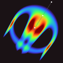
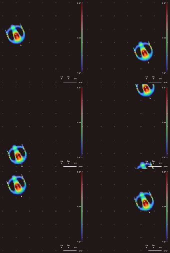
Lenia is a family of cellular automata created by Bert Wang-Chak Chan. It is intended to be a continuous generalization of Conway's Game of Life, with continuous states, space and time. As a consequence of its continuous, high-resolution domain, the complex autonomous patterns ("lifeforms" or "spaceships") generated in Lenia are described as differing from those appearing in other cellular automata, being "geometric, metameric, fuzzy, resilient, adaptive, and rule-generic".
Lenia won the 2018 Virtual Creatures Contest at the Genetic and Evolutionary Computation Conference in Kyoto, an honorable mention for the ALIFE Art Award at ALIFE 2018 in Tokyo, and Outstanding Publication of 2019 by the International Society for Artificial Life (ISAL).
Rules
Iterative updates
Let be the lattice or grid containing a set of states . Like many cellular automata, Lenia is updated iteratively; each output state is a pure function of the previous state, such that
where is the initial state and is the global rule, representing the application of the local rule over every site . Thus .
If the simulation is advanced by at each timestep, then the time resolution .
State sets
Let with maximum . This is the state set of the automaton and characterizes the possible states that may be found at each site. Larger correspond to higher state resolutions in the simulation. Many cellular automata use the lowest possible state resolution, i.e. . Lenia allows for much higher resolutions. Note that the actual value at each site is not in but rather an integer multiple of ; therefore we have for all . For example, given , .
Neighborhoods
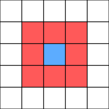

Mathematically, neighborhoods like those in Game of Life may be represented using a set of position vectors in . For the classic Moore neighborhood used by Game of Life, for instance, ; i.e. a square of size 3 centered on every site.
In Lenia's case, the neighborhood is instead a ball of radius centered on a site, , which may include the original site itself.
Note that the neighborhood vectors are not the absolute position of the elements, but rather a set of relative positions (deltas) with respect to any given site.
Local rule
There are discrete and continuous variants of Lenia. Let be a vector in within representing the position of a given site, and be the set of sites neighboring . Both variations comprise two stages:
- Using a convolution kernel to compute the potential distribution .
- Using a growth mapping to compute the final growth distribution .
Once is computed, it is scaled by the chosen time resolution and added to the original state value:Here, the clip function is defined by .
The local rules are defined as follows for discrete and continuous Lenia:
Kernel generation
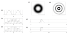
There are many ways to generate the convolution kernel . The final kernel is the composition of a kernel shell and a kernel skeleton .
For the kernel shell , Chan gives several functions that are defined radially. Kernel shell functions are unimodal and subject to the constraint (and typically as well). Example kernel functions include:
Here, is the indicator function.
Once the kernel shell has been defined, the kernel skeleton is used to expand it and compute the actual values of the kernel by transforming the shell into a series of concentric rings. The height of each ring is controlled by a kernel peak vector , where is the rank of the parameter vector. Then the kernel skeleton is defined as
The final kernel is therefore
such that is normalized to have an element sum of and (for conservation of mass). in the discrete case, and in the continuous case.
Growth mappings
The growth mapping , which is analogous to an activation function, may be any function that is unimodal, nonmonotonic, and accepts parameters . Examples include
where is a potential value drawn from .
Game of Life
The Game of Life may be regarded as a special case of discrete Lenia with . In this case, the kernel would be rectangular, with the functionand the growth rule also rectangular, with .
Patterns
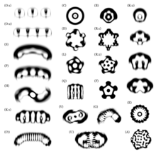
By varying the convolutional kernel, the growth mapping and the initial condition, over 400 "species" of "life" have been discovered in Lenia, displaying "self-organization, self-repair, bilateral and radial symmetries, locomotive dynamics, and sometimes chaotic nature". Chan has created a taxonomy for these patterns.
Related work

Other works have noted the strong similarity between cellular automata update rules and convolutions. Indeed, these works have focused on reproducing cellular automata using simplified convolutional neural networks. Mordvintsev et al. investigated the emergence of self-repairing pattern generation. Gilpin found that any cellular automaton could be represented as a convolutional neural network, and trained neural networks to reproduce existing cellular automata
In this light, cellular automata may be seen as a special case of recurrent convolutional neural networks. Lenia's update rule may also be seen as a single-layer convolution (the "potential field" ) with an activation function (the "growth mapping" ). However, Lenia uses far larger, fixed, kernels and is not trained via gradient descent.
See also
External links
- The Github repository for Lenia
- Chan's website for Lenia
- An invited seminar at Stanford given by Chan
References
- ^ Chan, Bert Wang-Chak (2019-10-15). "Lenia: Biology of Artificial Life". Complex Systems. 99999 (3): 251–286. arXiv:1812.05433. doi:10.25088/ComplexSystems.28.3.251.
- "Lenia". chakazul.github.io. Retrieved 2021-10-12.
- Roberts, Siobhan (2020-12-28). "The Lasting Lessons of John Conway's Game of Life". The New York Times. ISSN 0362-4331. Retrieved 2021-10-13.
- "The virtual creatures competition". virtualcreatures.github.io. Retrieved 2021-10-12.
- "ALife Art Award 2018". ALIFE Art Award 2018. Retrieved 2021-10-12.
- "2020 ISAL Awards: Winners".
- "Lenia". chakazul.github.io. Retrieved 2021-10-13.
- ^ Gilpin, William (2019-09-04). "Cellular automata as convolutional neural networks". Physical Review E. 100 (3): 032402. arXiv:1809.02942. doi:10.1103/PhysRevE.100.032402. ISSN 2470-0045.
- Mordvintsev, Alexander; Randazzo, Ettore; Niklasson, Eyvind; Levin, Michael (2020-02-11). "Growing Neural Cellular Automata". Distill. 5 (2): e23. doi:10.23915/distill.00023. ISSN 2476-0757.
| Conway's Game of Life and related cellular automata | |
|---|---|
| Structures | |
| Life variants | |
| Concepts | |
| Implementations | |
| Key people | |
| Websites | |
| Popular culture | |
 be the lattice or grid containing a set of states
  . Like many cellular automata, Lenia is updated iteratively; each output state is a
 is the initial state and
  is the global rule, representing the application of the local rule over every site
  . Thus
  .
.
 at each timestep, then the time resolution
  .
.
 with maximum
  . This is the state set of the automaton and characterizes the possible states that may be found at each site. Larger
  correspond to higher state resolutions in the simulation. Many cellular automata use the lowest possible state resolution, i.e.
  . Lenia allows for much higher resolutions. Note that the actual value at each site is not in
  but rather an integer multiple of
  ; therefore we have
  for all
  . For example, given
  ,
,  .
.
 . For the classic
  ; i.e. a square of size 3 centered on every site.
 centered on a site,
  , which may include the original site itself.
 be a vector in
  be the set of sites neighboring
  to compute the potential distribution
  .
. to compute the final growth distribution
  .
. is computed, it is scaled by the chosen time resolution
  Here, the clip function is defined by
  .
.

 . The final kernel is the composition of a kernel shell
  and a kernel skeleton
  .
.
 (and typically
  as well). Example kernel functions include:

 is the
  , where
  is the rank of the parameter vector. Then the kernel skeleton
 is therefore

 and
and  (for
(for  in the discrete case, and
  in the continuous case.
 . Examples include

 is a potential value drawn from
  .
.
 . In this case, the kernel would be rectangular, with the function
 and the growth rule also rectangular, with
  .
.
 ). However, Lenia uses far larger, fixed, kernels and is not trained via gradient descent.