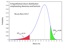
The Rachev Ratio (or R-Ratio) is a risk-return performance measure of an investment asset, portfolio, or strategy. It was devised by Dr. Svetlozar Rachev and has been extensively studied in quantitative finance. Unlike the reward-to-variability ratios, such as Sharpe ratio and Sortino ratio, the Rachev ratio is a reward-to-risk ratio, which is designed to measure the right tail reward potential relative to the left tail risk in a non-Gaussian setting. Intuitively, it represents the potential for extreme positive returns compared to the risk of extreme losses (negative returns), at a rarity frequency q (quantile level) defined by the user.
The ratio is defined as the Expected Tail Return (ETR) in the best q% cases divided by the Expected tail loss (ETL) in the worst q% cases. The ETL is the average loss incurred when losses exceed the Value at Risk at a predefined quantile level. The ETR, defined by symmetry to the ETL, is the average profit gained when profits exceed the Profit at risk at a predefined quantile level.
For more tailored applications, the generalized Rachev Ratio has been defined with different powers and/or different confidence levels of the ETR and ETL.
Definition
According to its original version introduced by the authors in 2004, the Rachev ratio is defined as:
or, alternatively,
where and belong to , and in the symmetric case: . is the risk-free rate of return and presents the portfolio return. The ETL is the expected tail loss, also known as conditional value at risk (CVaR), is defined as:
and
is the value at risk (VaR) of the random return .
Thus, the ETL can be interpreted as the average loss beyond VaR:
.
The generalized Rachev ratio is the ratio between the power CVaR of the opposite of the excess return at a given confidence level and the power CVaR of the excess return at another confidence level. That is,
where is the power CVaR of , and is a positive constant. The main advantage of the generalized Rachev ratio over the traditional Rachev ratio is conferred by the power indexes and that characterize an investor's aversion to risk.
Properties
The Rachev ratio can be used in both ex-ante and ex-post analyses.

In the ex-post analysis, the Rachev ratio is computed by dividing the corresponding two sample AVaR's. Since the performance levels in the Rachev ratio are quantiles of the active return distribution, they are relative levels as they adjust according to the distribution. For example, if the scale is small, then the two performance levels will be closer to each other. As a consequence, the Rachev ratio is always well-defined.
In the ex-ante analysis, optimal portfolio problems based on the Rachev ratio are, generally, numerically hard to solve because the Rachev ratio is a fraction of two CVaRs which are convex functions of portfolio weights. In effect, the Rachev ratio, if viewed as a function of portfolio weights, may have many local extrema.
Several empirical tests of the Rachev ratio and the generalized Rachev ratio have been proposed.
An algorithm for solving Rachev ratio optimization problem was provided in Konno, Tanaka, and Yamamoto (2011).
Example
In quantitative finance, non-Gaussian return distributions are common. The Rachev ratio, as a risk-adjusted performance measurement, characterizes the skewness and kurtosis of the return distribution (see picture on the right).
See also
- Post-modern portfolio theory
- Upside potential ratio
- Sharpe ratio
- Sortino ratio
- Omega ratio
- Modern Portfolio Theory
References
- ^ Biglova, Almira; Ortobelli, Sergio; Rachev, Svetlozar T.; Stoyanov, Stoyan (2004). "Different Approaches to Risk Estimation in Portfolio Theory". The Journal of Portfolio Management. 31. The Journal of Portfolio Management, Fall 2004, Vol. 31, No. 1: pp. 103-112: 103–112. doi:10.3905/jpm.2004.443328. S2CID 153594336.
- Fehr, Ben. "Beyond the Normal Distribution" (PDF). Frankfurter Allgemeine Zeitung. Archived from the original (PDF) on 1 September 2006. Retrieved 16 March 2006.
- Cheridito, P.; Kromer, E. (2013). "Reward-Risk Ratios". Journal of Investment Strategies. 3 (1): 3–18. doi:10.21314/JOIS.2013.022.
- ^ Farinelli, S.; Ferreira, M.; Rossello, D.; Thoeny, M.; Tibiletti, L. (2008). "Beyond Sharpe ratio: Optimal asset allocation using different performance ratios". Journal of Banking and Finance. 32 (10): 2057–2063. doi:10.1016/j.jbankfin.2007.12.026.
- Svetlozar Rachev. "Lecture 10: Performance measures" (PDF). stat.kit.edu. Retrieved 15 May 2024.
- Rachev, Svetlozar T.; Stoyanov, Stoyan V.; Fabozzi, Frank J. (2008). Advanced Stochastic Models, Risk Assessment, and Portfolio Optimization (1st ed.). Wiley. ISBN 978-0-470-05316-4.
- Satchell, Stephen (2009-10-22). Optimizing Optimization: The Next Generation of Optimization Applications and Theory (1st ed.). Academic Press. ISBN 9780750633611.
- Konno, Hiroshi; Tanaka, Katsuhiro; Yamamoto, Rei (2011). "Construction of a portfolio with shorter downside tail and longer upside tail". Computational Optimization and Applications. 48 (2): 199. doi:10.1007/s10589-009-9255-4. S2CID 29816889.


 and
and  belong to
  , and in the symmetric case:
  .
.  is the risk-free rate of return and
  presents the portfolio return. The ETL is the expected tail loss, also known as conditional value at risk (

 .
.
 .
.

 is the power CVaR of
  is a positive constant. The main advantage of the generalized Rachev ratio over the traditional Rachev ratio is conferred by the power indexes
  that characterize an investor's aversion to risk.