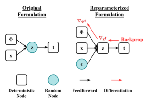
The reparameterization trick (aka "reparameterization gradient estimator") is a technique used in statistical machine learning, particularly in variational inference, variational autoencoders, and stochastic optimization. It allows for the efficient computation of gradients through random variables, enabling the optimization of parametric probability models using stochastic gradient descent, and the variance reduction of estimators.
It was developed in the 1980s in operations research, under the name of "pathwise gradients", or "stochastic gradients". Its use in variational inference was proposed in 2013.
Mathematics
Let be a random variable with distribution , where is a vector containing the parameters of the distribution.
REINFORCE estimator
Consider an objective function of the form:Without the reparameterization trick, estimating the gradient can be challenging, because the parameter appears in the random variable itself. In more detail, we have to statistically estimate:The REINFORCE estimator, widely used in reinforcement learning and especially policy gradient, uses the following equality:This allows the gradient to be estimated:The REINFORCE estimator has high variance, and many methods were developed to reduce its variance.
Reparameterization estimator
The reparameterization trick expresses as:Here, is a deterministic function parameterized by , and is a noise variable drawn from a fixed distribution . This gives:Now, the gradient can be estimated as:
Examples
For some common distributions, the reparameterization trick takes specific forms:
Normal distribution: For , we can use:
Exponential distribution: For , we can use:Discrete distribution can be reparameterized by the Gumbel distribution (Gumbel-softmax trick or "concrete distribution").
In general, any distribution that is differentiable with respect to its parameters can be reparameterized by inverting the multivariable CDF function, then apply the implicit method. See for an exposition and application to the Gamma Beta, Dirichlet, and von Mises distributions.
Applications
Variational autoencoder


In Variational Autoencoders (VAEs), the VAE objective function, known as the Evidence Lower Bound (ELBO), is given by:
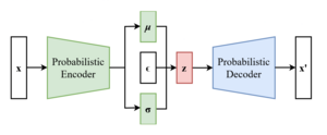
where is the encoder (recognition model), is the decoder (generative model), and is the prior distribution over latent variables. The gradient of ELBO with respect to is simplybut the gradient with respect to requires the trick. Express the sampling operation as:where and are the outputs of the encoder network, and denotes element-wise multiplication. Then we havewhere . This allows us to estimate the gradient using Monte Carlo sampling:where and for .
This formulation enables backpropagation through the sampling process, allowing for end-to-end training of the VAE model using stochastic gradient descent or its variants.
Variational inference
More generally, the trick allows using stochastic gradient descent for variational inference. Let the variational objective (ELBO) be of the form:Using the reparameterization trick, we can estimate the gradient of this objective with respect to :
Dropout
The reparameterization trick has been applied to reduce the variance in dropout, a regularization technique in neural networks. The original dropout can be reparameterized with Bernoulli distributions:where is the weight matrix, is the input, and are the (fixed) dropout rates.
More generally, other distributions can be used than the Bernoulli distribution, such as the gaussian noise:where and , with and being the mean and variance of the -th output neuron. The reparameterization trick can be applied to all such cases, resulting in the variational dropout method.
See also
References
- ^ Figurnov, Mikhail; Mohamed, Shakir; Mnih, Andriy (2018). "Implicit Reparameterization Gradients". Advances in Neural Information Processing Systems. 31. Curran Associates, Inc.
- Fu, Michael C. "Gradient estimation." Handbooks in operations research and management science 13 (2006): 575-616.
- Kingma, Diederik P.; Welling, Max (2022-12-10). "Auto-Encoding Variational Bayes". arXiv:1312.6114 .
- Williams, Ronald J. (1992-05-01). "Simple statistical gradient-following algorithms for connectionist reinforcement learning". Machine Learning. 8 (3): 229–256. doi:10.1007/BF00992696. ISSN 1573-0565.
- Greensmith, Evan; Bartlett, Peter L.; Baxter, Jonathan (2004). "Variance Reduction Techniques for Gradient Estimates in Reinforcement Learning". Journal of Machine Learning Research. 5 (Nov): 1471–1530. ISSN 1533-7928.
- Maddison, Chris J.; Mnih, Andriy; Teh, Yee Whye (2017-03-05). "The Concrete Distribution: A Continuous Relaxation of Discrete Random Variables". arXiv:1611.00712 .
- Kingma, Durk P; Salimans, Tim; Welling, Max (2015). "Variational Dropout and the Local Reparameterization Trick". Advances in Neural Information Processing Systems. 28. arXiv:1506.02557.
Further reading
- Ruiz, Francisco R.; AUEB, Titsias RC; Blei, David (2016). "The Generalized Reparameterization Gradient". Advances in Neural Information Processing Systems. 29. arXiv:1610.02287. Retrieved September 23, 2024.
- Zhang, Cheng; Butepage, Judith; Kjellstrom, Hedvig; Mandt, Stephan (2019-08-01). "Advances in Variational Inference". IEEE Transactions on Pattern Analysis and Machine Intelligence. 41 (8): 2008–2026. arXiv:1711.05597. doi:10.1109/TPAMI.2018.2889774. ISSN 0162-8828. PMID 30596568.
- Mohamed, Shakir (October 29, 2015). "Machine Learning Trick of the Day (4): Reparameterisation Tricks". The Spectator. Retrieved September 23, 2024.
 be a random variable with distribution
  , where
  is a vector containing the parameters of the distribution.
 Without the reparameterization trick, estimating the gradient
  can be challenging, because the parameter appears in the random variable itself. In more detail, we have to statistically estimate:
 The REINFORCE estimator, widely used in
  This allows the gradient to be estimated:
 The REINFORCE estimator has high variance, and many methods were developed to
  Here,
Here,  is a deterministic function parameterized by
  is a noise variable drawn from a fixed distribution
  . This gives:
 Now, the gradient can be estimated as:
 , we can use:
 , we can use:
 is injected into the latent space
 is the encoder (recognition model),
  is the decoder (generative model), and
  is the prior distribution over latent variables. The gradient of ELBO with respect to
  is simply
 but the gradient with respect to
  as:
as: where
where  and
and  are the outputs of the encoder network, and
  denotes
  where
where  . This allows us to estimate the gradient using Monte Carlo sampling:
 where
where  and
and  for
for  .
.
 Using the reparameterization trick, we can estimate the gradient of this objective with respect to
 where
where  is the weight matrix,
  is the input, and
  are the (fixed) dropout rates.
 where
where  and
and  , with
  and
and  being the mean and variance of the
  -th output neuron. The reparameterization trick can be applied to all such cases, resulting in the variational dropout method.