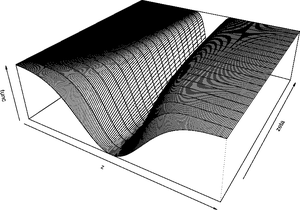
In statistics, Smooth Transition Autoregressive (STAR) models are typically applied to time series data as an extension of autoregressive models, in order to allow for higher degree of flexibility in model parameters through a smooth transition.
Given a time series of data xt, the STAR model is a tool for understanding and, perhaps, predicting future values in this series, assuming that the behaviour of the series changes depending on the value of the transition variable. The transition might depend on the past values of the x series (similar to the SETAR models), or exogenous variables.
The model consists of 2 autoregressive (AR) parts linked by the transition function. The model is usually referred to as the STAR(p) models proceeded by the letter describing the transition function (see below) and p is the order of the autoregressive part. Most popular transition function include exponential function and first and second-order logistic functions. They give rise to Logistic STAR (LSTAR) and Exponential STAR (ESTAR) models.
Definition
AutoRegressive Models
Consider a simple AR(p) model for a time series yt
where:
- for i=1,2,...,p are autoregressive coefficients, assumed to be constant over time;
- stands for white-noise error term with constant variance.
written in a following vector form:
where:
- is a column vector of variables;
- is the vector of parameters :;
- stands for white-noise error term with constant variance.

STAR as an Extension of the AutoRegressive Model
STAR models were introduced and comprehensively developed by Kung-sik Chan and Howell Tong in 1986 (esp. p. 187), in which the same acronym was used. It originally stands for Smooth Threshold AutoRegressive. For some background history, see Tong (2011, 2012). The models can be thought of in terms of extension of autoregressive models discussed above, allowing for changes in the model parameters according to the value of a transition variable zt. Chan and Tong (1986) rigorously proved that the family of STAR models includes the SETAR model as a limiting case by showing the uniform boundedness and equicontinuity with respect to the switching parameter. Without this proof, to say that STAR models nest the SETAR model lacks justification. Unfortunately, whether one should use a SETAR model or a STAR model for one's data has been a matter of subjective judgement, taste and inclination in much of the literature. Fortunately, the test procedure, based on David Cox's test of separate family of hypotheses and developed by Gao, Ling and Tong (2018, Statistica Sinica, volume 28, 2857-2883) is now available to address this issue. Such a test is important before adopting a STAR model because, among other issues, the parameter controlling its rate of switching is notoriously data-hungry.
Defined in this way, STAR model can be presented as follows:
where:
- is a column vector of variables;
- is the transition function bounded between 0 and 1.
Basic Structure
They can be understood as two-regime SETAR model with smooth transition between regimes, or as continuum of regimes. In both cases the presence of the transition function is the defining feature of the model as it allows for changes in values of the parameters.
Transition Function

Three basic transition functions and the name of resulting models are:
- first order logistic function - results in Logistic STAR (LSTAR) model:
- exponential function - results in Exponential STAR (ESTAR) model:
- second order logistic function:
See also
- Characterizations of the exponential function
- Exponential growth
- Exponentiation
- Generalised logistic function
- Logistic distribution
- SETAR (model)
References
| This article includes a list of references, related reading, or external links, but its sources remain unclear because it lacks inline citations. Please help improve this article by introducing more precise citations. (June 2012) (Learn how and when to remove this message) |
- Chan, K. S.; Tong, H. (1986). "On Estimating Thresholds in Autoregressive Models". Journal of Time Series Analysis. 7 (3): 178–190. doi:10.1111/j.1467-9892.1986.tb00501.x.
- Van Dijk, D.; Teräsvirta, T.; Franses, P. H. (2002). "Smooth Transition Autoregressive Models—A Survey of Recent Developments". Econometric Reviews. 21 (1): 1–47. doi:10.1081/ETC-120008723. hdl:1765/1656.
- Tong, H. (2011). "Threshold models in time series analysis—30 years on (with discussions by P. Whittle, M. Rosenblatt, B. E. Hansen, P. Brockwell, N. I. Samia & F. Battaglia)" (PDF). Statistics and Its Interface. 4 (2): 107–118. doi:10.4310/SII.2011.v4.n2.a1.
- Hansen, B. E. (2011). "Threshold Autoregression in Economics" (PDF). Statistics and Its Interface. 4 (2): 123–127. doi:10.4310/sii.2011.v4.n2.a4.
- Tong, H. (2012). "Discussion of 'An analysis of global warming in the Alpine region based on nonlinear nonstationary time series models' by Battaglia and Protopapa" (PDF). Statistical Methods and Applications. 21 (3): 335–339. doi:10.1007/s10260-012-0196-1.
 varying from -10 to +10 and
  - from 0 to 1.
 for i=1,2,...,p are
  stands for
 is a column vector of variables;
 is the vector of parameters :
 ;
; stands for
  and
and  ) equal to -7 and +3.
 is a column vector of variables;
 is the transition function bounded between 0 and 1.

