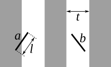
In probability theory, Buffon's needle problem is a question first posed in the 18th century by Georges-Louis Leclerc, Comte de Buffon:
- Suppose we have a floor made of parallel strips of wood, each the same width, and we drop a needle onto the floor. What is the probability that the needle will lie across a line between two strips?
Buffon's needle was the earliest problem in geometric probability to be solved; it can be solved using integral geometry. The solution for the sought probability p, in the case where the needle length l is not greater than the width t of the strips, is
This can be used to design a Monte Carlo method for approximating the number π, although that was not the original motivation for de Buffon's question. The seemingly unusual appearance of π in this expression occurs because the underlying probability distribution function for the needle orientation is rotationally symmetric.
Solution
The problem in more mathematical terms is: Given a needle of length l dropped on a plane ruled with parallel lines t units apart, what is the probability that the needle will lie across a line upon landing?
Let x be the distance from the center of the needle to the closest parallel line, and let θ be the acute angle between the needle and one of the parallel lines.
The uniform probability density function (PDF) of x between 0 and t/2 is
Here, x = 0 represents a needle that is centered directly on a line, and x = t/2 represents a needle that is perfectly centered between two lines. The uniform PDF assumes the needle is equally likely to fall anywhere in this range, but could not fall outside of it.
The uniform probability density function of θ between 0 and π/2 is
Here, θ = 0 represents a needle that is parallel to the marked lines, and θ = π/2 radians represents a needle that is perpendicular to the marked lines. Any angle within this range is assumed an equally likely outcome.
The two random variables, x and θ, are independent, so the joint probability density function is the product
The needle crosses a line if
Now there are two cases.
Case 1: Short needle (l ≤ t)
Integrating the joint probability density function gives the probability that the needle will cross a line:
Case 2: Long needle (l > t)
Suppose l > t. In this case, integrating the joint probability density function, we obtain:
where m(θ) is the minimum between l/2 sinθ and t/2.
Thus, performing the above integration, we see that, when l > t, the probability that the needle will cross at least one line is
or
In the second expression, the first term represents the probability of the angle of the needle being such that it will always cross at least one line. The right term represents the probability that the needle falls at an angle where its position matters, and it crosses the line.
Alternatively, notice that whenever θ has a value such that l sin θ ≤ t, that is, in the range 0 ≤ θ ≤ arcsin t/l, the probability of crossing is the same as in the short needle case. However if l sin θ > t, that is, arcsin t/l < θ ≤ π/2 the probability is constant and is equal to 1.
Using elementary calculus
The following solution for the "short needle" case, while equivalent to the one above, has a more visual flavor, and avoids iterated integrals.
We can calculate the probability P as the product of two probabilities: P = P1 · P2, where P1 is the probability that the center of the needle falls close enough to a line for the needle to possibly cross it, and P2 is the probability that the needle actually crosses the line, given that the center is within reach.
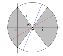
Looking at the illustration in the above section, it is apparent that the needle can cross a line if the center of the needle is within l/2 units of either side of the strip. Adding l/2 + l/2 from both sides and dividing by the whole width t, we obtain P1 = l/t.

Now, we assume that the center is within reach of the edge of the strip, and calculate P2. To simplify the calculation, we can assume that .
Let x and θ be as in the illustration in this section. Placing a needle's center at x, the needle will cross the vertical axis if it falls within a range of 2θ radians, out of π radians of possible orientations. This represents the gray area to the left of x in the figure. For a fixed x, we can express θ as a function of x: θ(x) = arccos(x). Now we can let x range from 0 to 1, and integrate:
Multiplying both results, we obtain P = P1 · P2 = l/t · 2/π = 2l/tπ as above.
There is an even more elegant and simple method of calculating the "short needle case". The end of the needle farthest away from any one of the two lines bordering its region must be located within a horizontal (perpendicular to the bordering lines) distance of l cos θ (where θ is the angle between the needle and the horizontal) from this line in order for the needle to cross it. The farthest this end of the needle can move away from this line horizontally in its region is t. The probability that the farthest end of the needle is located no more than a distance l cos θ away from the line (and thus that the needle crosses the line) out of the total distance t it can move in its region for 0 ≤ θ ≤ π/2 is given by
Without integrals
The short-needle problem can also be solved without any integration, in a way that explains the formula for p from the geometric fact that a circle of diameter t will cross the distance t strips always (i.e. with probability 1) in exactly two spots. This solution was given by Joseph-Émile Barbier in 1860 and is also referred to as "Buffon's noodle".
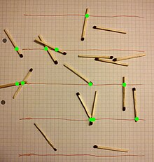
Estimating π

2l · n/th = 2 × 9 × 17/9 × 11 ≈ 3.1 ≈ π.

In the first, simpler case above, the formula obtained for the probability P can be rearranged to
Thus, if we conduct an experiment to estimate P, we will also have an estimate for π.
Suppose we drop n needles and find that h of those needles are crossing lines, so P is approximated by the fraction h/n. This leads to the formula:
In 1901, Italian mathematician Mario Lazzarini performed Buffon's needle experiment. Tossing a needle 3,408 times, he obtained the well-known approximation 355/113 for π, accurate to six decimal places. Lazzarini's "experiment" is an example of confirmation bias, as it was set up to replicate the already well-known approximation of 355/113 (in fact, there is no better rational approximation with fewer than five digits in the numerator and denominator, see also Milü), yielding a more accurate "prediction" of π than would be expected from the number of trials, as follows:
Lazzarini chose needles whose length was 5/6 of the width of the strips of wood. In this case, the probability that the needles will cross the lines is 5/3π. Thus if one were to drop n needles and get x crossings, one would estimate π as
So if Lazzarini was aiming for the result 355/113, he needed n and x such that
or equivalently,
To do this, one should pick n as a multiple of 213, because then 113n/213 is an integer; one then drops n needles, and hopes for exactly x = 113n/213 successes. If one drops 213 needles and happens to get 113 successes, then one can triumphantly report an estimate of π accurate to six decimal places. If not, one can just do 213 more trials and hope for a total of 226 successes; if not, just repeat as necessary. Lazzarini performed 3,408 = 213 × 16 trials, making it seem likely that this is the strategy he used to obtain his "estimate".
The above description of strategy might even be considered charitable to Lazzarini. A statistical analysis of intermediate results he reported for fewer tosses leads to a very low probability of achieving such close agreement to the expected value all through the experiment. This makes it very possible that the "experiment" itself was never physically performed, but based on numbers concocted from imagination to match statistical expectations, but too well, as it turns out.
Dutch science journalist Hans van Maanen argues, however, that Lazzarini's article was never meant to be taken too seriously as it would have been pretty obvious for the readers of the magazine (aimed at school teachers) that the apparatus that Lazzarini said to have built cannot possibly work as described.
Laplace's extension (short needle case)
Now consider the case where the plane contains two sets of parallel lines orthogonal to one another, creating a standard perpendicular grid. We aim to find the probability that the needle intersects at least one line on the grid. Let a and b be the sides of the rectangle that contains the midpoint of the needle whose length is l. Since this is the short needle case, l < a, l < b. Let (x,y) mark the coordinates of the needle's midpoint and let φ mark the angle formed by the needle and the x-axis. Similar to the examples described above, we consider x, y, φ to be independent uniform random variables over the ranges 0 ≤ x ≤ a, 0 ≤ y ≤ b, −π/2 ≤ φ ≤ π/2.
To solve such a problem, we first compute the probability that the needle crosses no lines, and then we take its complement. We compute this first probability by determining the volume of the domain where the needle crosses no lines and then divide that by the volume of all possibilities, V. We can easily see that V = πab.
Now let V* be the volume of possibilities where the needle does not intersect any line. Developed by J.V. Uspensky,
where F(φ) is the region where the needle does not intersect any line given an angle φ. To determine F(φ), let's first look at the case for the horizontal edges of the bounding rectangle. The total side length is a and the midpoint must not be within l/2 cos φ of either endpoint of the edge. Thus, the total allowable length for no intersection is a − 2(l/2 cos φ) or simply just a − l cos φ. Equivalently, for the vertical edges with length b, we have b ± l sin φ. The ± accounts for the cases where φ is positive or negative. Taking the positive case and then adding the absolute value signs in the final answer for generality, we get
Now we can compute the following integral:
Thus, the probability that the needle does not intersect any line is
And finally, if we want to calculate the probability, P, that the needle does intersect at least one line, we need to subtract the above result from 1 to compute its compliment, yielding
- .
Comparing estimators of π
As mentioned above, Buffon's needle experiment can be used to estimate π. This fact holds for Laplace's extension too since π shows up in that answer as well. The following question then naturally arises and is discussed by E.F. Schuster in 1974. Is Buffon's experiment or Laplace's a better estimator of the value of π? Since in Laplace's extension there are two sets of parallel lines, we compare N drops when there is a grid (Laplace), and 2N drops in Buffon's original experiment.
Let A be the event that the needle intersects a horizontal line (parallel to the x-axis)
and let B be the event that the needle intersects a vertical line (parallel to the y-axis)
For simplicity in the algebraic formulation ahead, let a = b = t = 2l such that the original result in Buffon's problem is P(A) = P(B) = 1/π. Furthermore, let N = 100 drops.
Now let us examine P(AB) for Laplace's result, that is, the probability the needle intersects both a horizontal and a vertical line. We know that
From the above section, P(A′B′), or the probability that the needle intersects no lines is
We can solve for P(A′B) and P(AB′) using the following method:
Solving for P(A′B) and P(AB′) and plugging that into the original definition for P(AB) a few lines above, we get
Although not necessary to the problem, it is now possible to see that P(A′B) = P(AB′) = 3/4π. With the values above, we are now able to determine which of these estimators is a better estimator for π. For the Laplace variant, let p̂ be the estimator for the probability that there is a line intersection such that
- .
We are interested in the variance of such an estimator to understand the usefulness or efficiency of it. To compute the variance of p̂, we first compute Var(xn + yn) where
Solving for each part individually,
We know from the previous section that
yielding
Thus,
Returning to the original problem of this section, the variance of estimator p̂ is
Now let us calculate the number of drops, M, needed to achieve the same variance as 100 drops over perpendicular lines. If M < 200 then we can conclude that the setup with only parallel lines is more efficient than the case with perpendicular lines. Conversely if M is equal to or more than 200, than Buffon's experiment is equally or less efficient, respectively. Let q̂ be the estimator for Buffon's original experiment. Then,
and
Solving for M,
Thus, it takes 222 drops with only parallel lines to have the same certainty as 100 drops in Laplace's case. This isn't actually surprising because of the observation that Cov(xn,yn) < 0. Because xn and yn are negatively correlated random variables, they act to reduce the total variance in the estimator that is an average of the two of them. This method of variance reduction is known as the antithetic variates method.
See also
References
- Histoire de l'Acad. Roy. des. Sciences (1733), 43–45; Histoire naturelle, générale et particulière Supplément 4 (1777), p. 46.
- Seneta, Eugene; Parshall, Karen Hunger; Jongmans, François (2001). "Nineteenth-Century Developments in Geometric Probability: J. J. Sylvester, M. W. Crofton, J.-É. Barbier, and J. Bertrand". Archive for History of Exact Sciences. 55 (6): 501–524. doi:10.1007/s004070100038. ISSN 0003-9519. JSTOR 41134124. S2CID 124429237.
- Behrends, Ehrhard. "Buffon: Hat er Stöckchen geworfen oder hat er nicht?" (PDF). Retrieved 14 March 2015.
- The problem formulation here avoids having to work with Regular conditional probability densities.
- Aigner, Martin; Ziegler, Günter M. (2013). Proofs from THE BOOK (2nd ed.). Springer Science & Business Media. pp. 189–192.
- Lazzarini, M. (1901). "Un'applicazione del calcolo della probabilità alla ricerca sperimentale di un valore approssimato di π" [An Application of Probability Theory to Experimental Research of an Approximation of π]. Periodico di Matematica per l'Insegnamento Secondario (in Italian). 4: 140–143.
- ^ Lee Badger, 'Lazzarini's Lucky Approximation of π', Mathematics Magazine 67, 1994, 83–91.
- Hans van Maanen, 'Het stokje van Lazzarini' (Lazzarini's stick), "Skepter" 31.3, 2018.
- J.V. Uspensky, 'Introduction to Mathematical Probability', 1937, 255.
- E. F. Schuster, Buffon's Needle Experiment, The American Mathematical Monthly, 1974, 29-29.
Bibliography
- Badger, Lee (April 1994). "Lazzarini's Lucky Approximation of π". Mathematics Magazine. 67 (2). Mathematical Association of America: 83–91. doi:10.2307/2690682. JSTOR 2690682.
- Ramaley, J. F. (October 1969). "Buffon's Noodle Problem". The American Mathematical Monthly. 76 (8). Mathematical Association of America: 916–918. doi:10.2307/2317945. JSTOR 2317945.
- Mathai, A. M. (1999). An Introduction to Geometrical Probability. Newark: Gordon & Breach. p. 5. ISBN 978-90-5699-681-9.
- Dell, Zachary; Franklin, Scott V. (September 2009). "The Buffon-Laplace needle problem in three dimensions". Journal of Statistical Mechanics: Theory and Experiment. 2009 (9): 010. Bibcode:2009JSMTE..09..010D. doi:10.1088/1742-5468/2009/09/P09010. S2CID 32470555.
- Schroeder, L. (1974). "Buffon's needle problem: An exciting application of many mathematical concepts". Mathematics Teacher, 67 (2), 183–6.
- Uspensky, James Victor. "Introduction to mathematical probability." (1937).
External links
- Buffon's Needle Problem at cut-the-knot
- Math Surprises: Buffon's Noodle at cut-the-knot
- MSTE: Buffon's Needle
- Buffon's Needle Java Applet
- Estimating PI Visualization (Flash)
- Buffon's needle: fun and fundamentals (presentation) at slideshare
- Animations for the Simulation of Buffon's Needle by Yihui Xie using the R package animation
- 3D Physical Animation by Jeffrey Ventrella
- Padilla, Tony. "π Pi and Buffon's Needle". Numberphile. Brady Haran. Archived from the original on 2013-05-17. Retrieved 2013-04-09.


 .
.


 .
.


 .
.


