Ensemble of states at a constant temperature
| Statistical mechanics |
|---|
 |
| Particle statistics |
Thermodynamic ensembles
|
| Models |
| Potentials |
| Scientists |
In statistical mechanics, a canonical ensemble is the statistical ensemble that represents the possible states of a mechanical system in thermal equilibrium with a heat bath at a fixed temperature. The system can exchange energy with the heat bath, so that the states of the system will differ in total energy.
The principal thermodynamic variable of the canonical ensemble, determining the probability distribution of states, is the absolute temperature (symbol: T). The ensemble typically also depends on mechanical variables such as the number of particles in the system (symbol: N) and the system's volume (symbol: V), each of which influence the nature of the system's internal states. An ensemble with these three parameters, which are assumed constant for the ensemble to be considered canonical, is sometimes called the NVT ensemble.
The canonical ensemble assigns a probability P to each distinct microstate given by the following exponential:
where E is the total energy of the microstate, and k is the Boltzmann constant.
The number F is the free energy (specifically, the Helmholtz free energy) and is assumed to be a constant for a specific ensemble to be considered canonical. However, the probabilities and F will vary if different N, V, T are selected. The free energy F serves two roles: first, it provides a normalization factor for the probability distribution (the probabilities, over the complete set of microstates, must add up to one); second, many important ensemble averages can be directly calculated from the function F(N, V, T).
An alternative but equivalent formulation for the same concept writes the probability as
using the canonical partition function
rather than the free energy. The equations below (in terms of free energy) may be restated in terms of the canonical partition function by simple mathematical manipulations.
Historically, the canonical ensemble was first described by Boltzmann (who called it a holode) in 1884 in a relatively unknown paper. It was later reformulated and extensively investigated by Gibbs in 1902.
Applicability of canonical ensemble
The canonical ensemble is the ensemble that describes the possible states of a system that is in thermal equilibrium with a heat bath (the derivation of this fact can be found in Gibbs).
The canonical ensemble applies to systems of any size; while it is necessary to assume that the heat bath is very large (i.e., take a macroscopic limit), the system itself may be small or large.
The condition that the system is mechanically isolated is necessary in order to ensure it does not exchange energy with any external object besides the heat bath. In general, it is desirable to apply the canonical ensemble to systems that are in direct contact with the heat bath, since it is that contact that ensures the equilibrium. In practical situations, the use of the canonical ensemble is usually justified either 1) by assuming that the contact is mechanically weak, or 2) by incorporating a suitable part of the heat bath connection into the system under analysis, so that the connection's mechanical influence on the system is modeled within the system.
When the total energy is fixed but the internal state of the system is otherwise unknown, the appropriate description is not the canonical ensemble but the microcanonical ensemble. For systems where the particle number is variable (due to contact with a particle reservoir), the correct description is the grand canonical ensemble. In statistical physics textbooks for interacting particle systems the three ensembles are assumed to be thermodynamically equivalent: the fluctuations of macroscopic quantities around their average value become small and, as the number of particles tends to infinity, they tend to vanish. In the latter limit, called the thermodynamic limit, the average constraints effectively become hard constraints. The assumption of ensemble equivalence dates back to Gibbs and has been verified for some models of physical systems with short-range interactions and subject to a small number of macroscopic constraints. Despite the fact that many textbooks still convey the message that ensemble equivalence holds for all physical systems, over the last decades various examples of physical systems have been found for which breaking of ensemble equivalence occurs.
Properties
- Uniqueness: The canonical ensemble is uniquely determined for a given physical system at a given temperature, and does not depend on arbitrary choices such as choice of coordinate system (classical mechanics), or basis (quantum mechanics), or of the zero of energy. The canonical ensemble is the only ensemble with constant N, V, and T that reproduces the fundamental thermodynamic relation.
- Statistical equilibrium (steady state): A canonical ensemble does not evolve over time, despite the fact that the underlying system is in constant motion. This is because the ensemble is only a function of a conserved quantity of the system (energy).
- Thermal equilibrium with other systems: Two systems, each described by a canonical ensemble of equal temperature, brought into thermal contact will each retain the same ensemble and the resulting combined system is described by a canonical ensemble of the same temperature.
- Maximum entropy: For a given mechanical system (fixed N, V), the canonical ensemble average −⟨log P⟩ (the entropy) is the maximum possible of any ensemble with the same ⟨E⟩.
- Minimum free energy: For a given mechanical system (fixed N, V) and given value of T, the canonical ensemble average ⟨E + kT log P⟩ (the Helmholtz free energy) is the lowest possible of any ensemble. This is easily seen to be equivalent to maximizing the entropy.
Free energy, ensemble averages, and exact differentials
- The partial derivatives of the function F(N, V, T) give important canonical ensemble average quantities:
- the average pressure is
- the Gibbs entropy is
- the partial derivative ∂F/∂N is approximately related to chemical potential, although the concept of chemical equilibrium does not exactly apply to canonical ensembles of small systems.
- and the average energy is
- Exact differential: From the above expressions, it can be seen that the function F(V, T), for a given N, has the exact differential
- First law of thermodynamics: Substituting the above relationship for ⟨E⟩ into the exact differential of F, an equation similar to the first law of thermodynamics is found, except with average signs on some of the quantities:
- Energy fluctuations: The energy in the system has uncertainty in the canonical ensemble. The variance of the energy is
Example ensembles
"We may imagine a great number of systems of the same nature, but differing in the configurations and velocities which they have at a given instant, and differing in not merely infinitesimally, but it may be so as to embrace every conceivable combination of configuration and velocities..." J. W. Gibbs (1903)
Boltzmann distribution (separable system)
If a system described by a canonical ensemble can be separated into independent parts (this happens if the different parts do not interact), and each of those parts has a fixed material composition, then each part can be seen as a system unto itself and is described by a canonical ensemble having the same temperature as the whole. Moreover, if the system is made up of multiple similar parts, then each part has exactly the same distribution as the other parts.
In this way, the canonical ensemble provides exactly the Boltzmann distribution (also known as Maxwell–Boltzmann statistics) for systems of any number of particles. In comparison, the justification of the Boltzmann distribution from the microcanonical ensemble only applies for systems with a large number of parts (that is, in the thermodynamic limit).
The Boltzmann distribution itself is one of the most important tools in applying statistical mechanics to real systems, as it massively simplifies the study of systems that can be separated into independent parts (e.g., particles in a gas, electromagnetic modes in a cavity, molecular bonds in a polymer).
Ising model (strongly interacting system)
Main article: Ising modelIn a system composed of pieces that interact with each other, it is usually not possible to find a way to separate the system into independent subsystems as done in the Boltzmann distribution. In these systems it is necessary to resort to using the full expression of the canonical ensemble in order to describe the thermodynamics of the system when it is thermostatted to a heat bath. The canonical ensemble is generally the most straightforward framework for studies of statistical mechanics and even allows one to obtain exact solutions in some interacting model systems.
A classic example of this is the Ising model, which is a widely discussed toy model for the phenomena of ferromagnetism and of self-assembled monolayer formation, and is one of the simplest models that shows a phase transition. Lars Onsager famously calculated exactly the free energy of an infinite-sized square-lattice Ising model at zero magnetic field, in the canonical ensemble.
Precise expressions for the ensemble
The precise mathematical expression for a statistical ensemble depends on the kind of mechanics under consideration—quantum or classical—since the notion of a "microstate" is considerably different in these two cases. In quantum mechanics, the canonical ensemble affords a simple description since diagonalization provides a discrete set of microstates with specific energies. The classical mechanical case is more complex as it involves instead an integral over canonical phase space, and the size of microstates in phase space can be chosen somewhat arbitrarily.
Quantum mechanical
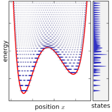
Example of canonical ensemble for a quantum system consisting of one particle in a potential well. Plot of all possible states of this system. The available stationary states displayed as horizontal bars of varying darkness according to |ψi(x)|.
 A canonical ensemble for this system, for the temperature shown. The states are weighted exponentially in energy.The particle's Hamiltonian is Schrödinger-type, Ĥ = U(x) + p/2m (the potential U(x) is plotted as a red curve). Each panel shows an energy-position plot with the various stationary states, along with a side plot showing the distribution of states in energy.
Further information on the representation of ensembles in quantum mechanics: Statistical ensemble (mathematical physics)
A statistical ensemble in quantum mechanics is represented by a density matrix, denoted by . In basis-free notation, the canonical ensemble is the density matrix
where Ĥ is the system's total energy operator (Hamiltonian), and exp() is the matrix exponential operator. The free energy F is determined by the probability normalization condition that the density matrix has a trace of one, :
The canonical ensemble can alternatively be written in a simple form using bra–ket notation, if the system's energy eigenstates and energy eigenvalues are known. Given a complete basis of energy eigenstates |ψi⟩, indexed by i, the canonical ensemble is:
where the Ei are the energy eigenvalues determined by Ĥ|ψi⟩ = Ei|ψi⟩. In other words, a set of microstates in quantum mechanics is given by a complete set of stationary states. The density matrix is diagonal in this basis, with the diagonal entries each directly giving a probability.
Classical mechanical
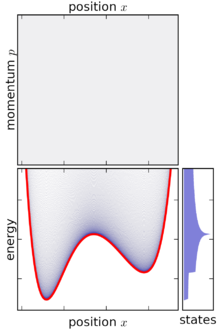
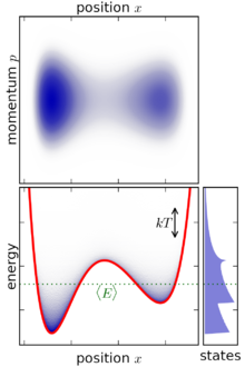
Example of canonical ensemble for a classical system consisting of one particle in a potential well. Plot of all possible states of this system. The available physical states are evenly distributed in phase space, but with an uneven distribution in energy; the side-plot displays dv/dE.
 A canonical ensemble for this system, for the temperature shown. The states are weighted exponentially in energy.Each panel shows phase space (upper graph) and energy-position space (lower graph). The particle's Hamiltonian is H = U(x) + p/2m, with the potential U(x) shown as a red curve. The side plot shows the distribution of states in energy.
Further information on the representation of ensembles in classical mechanics: Statistical ensemble (mathematical physics)
In classical mechanics, a statistical ensemble is instead represented by a joint probability density function in the system's phase space, ρ(p1, … pn, q1, … qn), where the p1, … pn and q1, … qn are the canonical coordinates (generalized momenta and generalized coordinates) of the system's internal degrees of freedom. In a system of particles, the number of degrees of freedom n depends on the number of particles N in a way that depends on the physical situation. For a three-dimensional monoatomic gas (not molecules), n = 3N. In diatomic gases there will also be rotational and vibrational degrees of freedom.
The probability density function for the canonical ensemble is:
where
- E is the energy of the system, a function of the phase (p1, … qn),
- h is an arbitrary but predetermined constant with the units of energy×time, setting the extent of one microstate and providing correct dimensions to ρ.
- C is an overcounting correction factor, often used for particle systems where identical particles are able to change place with each other.
- F provides a normalizing factor and is also the characteristic state function, the free energy.
Again, the value of F is determined by demanding that ρ is a normalized probability density function:
This integral is taken over the entire phase space.
In other words, a microstate in classical mechanics is a phase space region, and this region has volume hC. This means that each microstate spans a range of energy, however this range can be made arbitrarily narrow by choosing h to be very small. The phase space integral can be converted into a summation over microstates, once phase space has been finely divided to a sufficient degree.
See also
Notes
- Thermal contact means that the systems are made able to exchange energy through an interaction. The interaction must be weak as to not significantly disturb the systems' microstates.
- Since N is an integer, this "derivative" actually refers to a finite difference expression such as F(N) − F(N − 1), or F(N + 1) − F(N), or /2. These finite difference expressions are equivalent only in the thermodynamic limit (very large N).
- (Historical note) Gibbs' original ensemble effectively set h = 1 ×, leading to unit-dependence in the values of some thermodynamic quantities like entropy and chemical potential. Since the advent of quantum mechanics, h is often taken to be equal to the Planck constant in order to obtain a semiclassical correspondence with quantum mechanics.
- In a system of N identical particles, C = N! (factorial of N). This factor corrects the overcounting in phase space due to identical physical states being found in multiple locations. See the statistical ensemble article for more information on this overcounting.
References
- ^ Gibbs, Josiah Willard (1902). Elementary Principles in Statistical Mechanics. New York: Charles Scribner's Sons.
- Cercignani, Carlo (1998). Ludwig Boltzmann: The Man Who Trusted Atoms. Oxford University Press. ISBN 9780198501541.
- Roccaverde, Andrea (August 2018). "Is breaking of ensemble equivalence monotone in the number of constraints?". Indagationes Mathematicae. 30: 7–25. arXiv:1807.02791. doi:10.1016/j.indag.2018.08.001. ISSN 0019-3577. S2CID 119173928.
- Garlaschelli, Diego; den Hollander, Frank; Roccaverde, Andrea (November 25, 2016). "Ensemble nonequivalence in random graphs with modular structure". Journal of Physics A: Mathematical and Theoretical. 50 (1): 015001. arXiv:1603.08759. doi:10.1088/1751-8113/50/1/015001. ISSN 1751-8113. S2CID 53578783.
- Garlaschelli, Diego; den Hollander, Frank; Roccaverde, Andrea (July 13, 2018). "Covariance Structure Behind Breaking of Ensemble Equivalence in Random Graphs". Journal of Statistical Physics. 173 (3–4): 644–662. arXiv:1711.04273. Bibcode:2018JSP...173..644G. doi:10.1007/s10955-018-2114-x. ISSN 0022-4715. S2CID 52569377.
- Hollander, F. den; Mandjes, M.; Roccaverde, A.; Starreveld, N. J. (2018). "Ensemble equivalence for dense graphs". Electronic Journal of Probability. 23. arXiv:1703.08058. doi:10.1214/18-EJP135. ISSN 1083-6489. S2CID 53610196.
- Ellis, Richard S.; Haven, Kyle; Turkington, Bruce (2002). "Nonequivalent statistical equilibrium ensembles and refined stability theorems for most probable flows". Nonlinearity. 15 (2): 239. arXiv:math-ph/0012022. Bibcode:2002Nonli..15..239E. doi:10.1088/0951-7715/15/2/302. ISSN 0951-7715. S2CID 18616132.
- Barré, Julien; Gonçalves, Bruno (December 2007). "Ensemble inequivalence in random graphs". Physica A: Statistical Mechanics and Its Applications. 386 (1): 212–218. arXiv:0705.2385. Bibcode:2007PhyA..386..212B. doi:10.1016/j.physa.2007.08.015. ISSN 0378-4371. S2CID 15399624.
- Gao, Xiang (March 2022). "The Mathematics of the Ensemble Theory". Results in Physics. 34: 105230. arXiv:2006.00485. Bibcode:2022ResPh..3405230G. doi:10.1016/j.rinp.2022.105230. S2CID 221978379.
- Gibbs, J.W. (1928). The Collected Works, Vol. 2. Green & Co, London, New York: Longmans.
- Baxter, Rodney J. (1982). Exactly solved models in statistical mechanics. Academic Press Inc. ISBN 9780120831807.
- Onsager, L. (1944). "Crystal Statistics. I. A Two-Dimensional Model with an Order-Disorder Transition". Physical Review. 65 (3–4): 117–149. Bibcode:1944PhRv...65..117O. doi:10.1103/PhysRev.65.117.
| Statistical mechanics | ||
|---|---|---|
| Theory | ||
| Statistical thermodynamics | ||
| Models | ||
| Mathematical approaches | ||
| Critical phenomena | ||
| Entropy | ||
| Applications | ||


 . In basis-free notation, the canonical ensemble is the density matrix

 :
:


