This article has multiple issues. Please help improve it or discuss these issues on the talk page. (Learn how and when to remove these messages)
|

A Google matrix is a particular stochastic matrix that is used by Google's PageRank algorithm. The matrix represents a graph with edges representing links between pages. The PageRank of each page can then be generated iteratively from the Google matrix using the power method. However, in order for the power method to converge, the matrix must be stochastic, irreducible and aperiodic.
Adjacency matrix A and Markov matrix S
In order to generate the Google matrix G, we must first generate an adjacency matrix A which represents the relations between pages or nodes.
Assuming there are N pages, we can fill out A by doing the following:
- A matrix element is filled with 1 if node has a link to node , and 0 otherwise; this is the adjacency matrix of links.
- A related matrix S corresponding to the transitions in a Markov chain of given network is constructed from A by dividing the elements of column "j" by a number of where is the total number of outgoing links from node j to all other nodes. The columns having zero matrix elements, corresponding to dangling nodes, are replaced by a constant value 1/N. Such a procedure adds a link from every sink, dangling state to every other node.
- Now by the construction the sum of all elements in any column of matrix S is equal to unity. In this way the matrix S is mathematically well defined and it belongs to the class of Markov chains and the class of Perron-Frobenius operators. That makes S suitable for the PageRank algorithm.
Construction of Google matrix G

Then the final Google matrix G can be expressed via S as:
By the construction the sum of all non-negative elements inside each matrix column is equal to unity. The numerical coefficient is known as a damping factor.
Usually S is a sparse matrix and for modern directed networks it has only about ten nonzero elements in a line or column, thus only about 10N multiplications are needed to multiply a vector by matrix G.
Examples of Google matrix
An example of the matrix construction via Eq.(1) within a simple network is given in the article CheiRank.
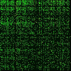
For the actual matrix, Google uses a damping factor around 0.85. The term gives a surfer probability to jump randomly on any page. The matrix belongs to the class of Perron-Frobenius operators of Markov chains. The examples of Google matrix structure are shown in Fig.1 for Misplaced Pages articles hyperlink network in 2009 at small scale and in Fig.2 for University of Cambridge network in 2006 at large scale.
Spectrum and eigenstates of G matrix

For there is only one maximal eigenvalue with the corresponding right eigenvector which has non-negative elements which can be viewed as stationary probability distribution. These probabilities ordered by their decreasing values give the PageRank vector with the PageRank used by Google search to rank webpages. Usually one has for the World Wide Web that with . The number of nodes with a given PageRank value scales as with the exponent . The left eigenvector at has constant matrix elements. With all eigenvalues move as except the maximal eigenvalue , which remains unchanged. The PageRank vector varies with but other eigenvectors with remain unchanged due to their orthogonality to the constant left vector at . The gap between and other eigenvalue being gives a rapid convergence of a random initial vector to the PageRank approximately after 50 multiplications on matrix.

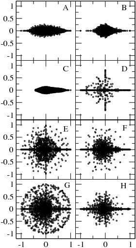
At the matrix has generally many degenerate eigenvalues (see e.g. ). Examples of the eigenvalue spectrum of the Google matrix of various directed networks is shown in Fig.3 from and Fig.4 from.
The Google matrix can be also constructed for the Ulam networks generated by the Ulam method for dynamical maps. The spectral properties of such matrices are discussed in . In a number of cases the spectrum is described by the fractal Weyl law .


The Google matrix can be constructed also for other directed networks, e.g. for the procedure call network of the Linux Kernel software introduced in . In this case the spectrum of is described by the fractal Weyl law with the fractal dimension (see Fig.5 from ). Numerical analysis shows that the eigenstates of matrix are localized (see Fig.6 from ). Arnoldi iteration method allows to compute many eigenvalues and eigenvectors for matrices of rather large size .
Other examples of matrix include the Google matrix of brain and business process management , see also. Applications of Google matrix analysis to DNA sequences is described in . Such a Google matrix approach allows also to analyze entanglement of cultures via ranking of multilingual Misplaced Pages articles abouts persons
Historical notes
The Google matrix with damping factor was described by Sergey Brin and Larry Page in 1998 , see also articles on PageRank history ,.
See also
- CheiRank
- Arnoldi iteration
- Markov chain
- Transfer operator
- Perron–Frobenius theorem
- Web search engines
References
- ^ Ermann, L.; Chepelianskii, A. D.; Shepelyansky, D. L. (2011). "Towards two-dimensional search engines". Journal of Physics A. 45 (27): 275101. arXiv:1106.6215. Bibcode:2012JPhA...45A5101E. doi:10.1088/1751-8113/45/27/275101. S2CID 14827486.
- ^ Langville, Amy N.; Meyer, Carl (2006). Google's PageRank and Beyond. Princeton University Press. ISBN 978-0-691-12202-1.
- ^ Austin, David (2008). "How Google Finds Your Needle in the Web's Haystack". AMS Feature Columns.
- Law, Edith (2008-10-09). "PageRank Lecture 12" (PDF).
- ^ Frahm, K. M.; Georgeot, B.; Shepelyansky, D. L. (2011-11-01). "Universal emergence of PageRank". Journal of Physics A. 44 (46): 465101. arXiv:1105.1062. Bibcode:2011JPhA...44T5101F. doi:10.1088/1751-8113/44/46/465101. S2CID 16292743.
- Donato, Debora; Laura, Luigi; Leonardi, Stefano; Millozzi, Stefano (2004-03-30). "Large scale properties of the Webgraph" (PDF). European Physical Journal B. 38 (2): 239–243. Bibcode:2004EPJB...38..239D. CiteSeerX 10.1.1.104.2136. doi:10.1140/epjb/e2004-00056-6. S2CID 10640375.
- Pandurangan, Gopal; Ranghavan, Prabhakar; Upfal, Eli (2005). "Using PageRank to Characterize Web Structure" (PDF). Internet Mathematics. 3 (1): 1–20. doi:10.1080/15427951.2006.10129114. S2CID 101281.
- ^ Georgeot, Bertrand; Giraud, Olivier; Shepelyansky, Dima L. (2010-05-25). "Spectral properties of the Google matrix of the World Wide Web and other directed networks". Physical Review E. 81 (5): 056109. arXiv:1002.3342. Bibcode:2010PhRvE..81e6109G. doi:10.1103/PhysRevE.81.056109. PMID 20866299. S2CID 14490804.
- ^ Ermann, L.; Chepelianskii, A. D.; Shepelyansky, D. L. (2011). "Fractal Weyl law for Linux Kernel Architecture". European Physical Journal B. 79 (1): 115–120. arXiv:1005.1395. Bibcode:2011EPJB...79..115E. doi:10.1140/epjb/e2010-10774-7. S2CID 445348.
- Serra-Capizzano, Stefano (2005). "Jordan Canonical Form of the Google Matrix: a Potential Contribution to the PageRank Computation". SIAM J. Matrix Anal. Appl. 27 (2): 305. doi:10.1137/s0895479804441407. hdl:11383/1494937.
- Ulam, Stanislaw (1960). A Collection of Mathematical Problems. Interscience Tracts in Pure and Applied Mathematics. New York: Interscience. p. 73.
- Froyland G.; Padberg K. (2009). "Almost-invariant sets and invariant manifolds—Connecting probabilistic and geometric descriptions of coherent structures in flows". Physica D. 238 (16): 1507. Bibcode:2009PhyD..238.1507F. doi:10.1016/j.physd.2009.03.002.
- Shepelyansky D.L.; Zhirov O.V. (2010). "Google matrix, dynamical attractors and Ulam networks". Phys. Rev. E. 81 (3): 036213. arXiv:0905.4162. Bibcode:2010PhRvE..81c6213S. doi:10.1103/physreve.81.036213. PMID 20365838. S2CID 15874766.
- Ermann L.; Shepelyansky D.L. (2010). "Google matrix and Ulam networks of intermittency maps". Phys. Rev. E. 81 (3): 036221. arXiv:0911.3823. Bibcode:2010PhRvE..81c6221E. doi:10.1103/physreve.81.036221. PMID 20365846. S2CID 388806.
- Ermann L.; Shepelyansky D.L. (2010). "Ulam method and fractal Weyl law for Perron-Frobenius operators". Eur. Phys. J. B. 75 (3): 299–304. arXiv:0912.5083. Bibcode:2010EPJB...75..299E. doi:10.1140/epjb/e2010-00144-0. S2CID 54899977.
- Frahm K.M.; Shepelyansky D.L. (2010). "Ulam method for the Chirikov standard map". Eur. Phys. J. B. 76 (1): 57–68. arXiv:1004.1349. Bibcode:2010EPJB...76...57F. doi:10.1140/epjb/e2010-00190-6. S2CID 55539783.
- Chepelianskii, Alexei D. (2010). "Towards physical laws for software architecture". arXiv:1003.5455 .
- Shepelyansky D.L.; Zhirov O.V. (2010). "Towards Google matrix of brain". Phys. Lett. A. 374 (31–32): 3206. arXiv:1002.4583. Bibcode:2010PhLA..374.3206S. doi:10.1016/j.physleta.2010.06.007.
- Abel M.; Shepelyansky D.L. (2011). "Google matrix of business process management". Eur. Phys. J. B. 84 (4): 493. arXiv:1009.2631. Bibcode:2011EPJB...84..493A. doi:10.1140/epjb/e2010-10710-y. S2CID 15510734.
- Kandiah, Vivek; Shepelyansky, Dima L. (2013). "Google Matrix Analysis of DNA Sequences". PLOS ONE. 8 (5): e61519. arXiv:1301.1626. Bibcode:2013PLoSO...861519K. doi:10.1371/journal.pone.0061519. PMC 3650020. PMID 23671568.
- Eom, Young-Ho; Shepelyansky, Dima L. (2013). "Highlighting Entanglement of Cultures via Ranking of Multilingual Misplaced Pages Articles". PLOS ONE. 8 (10): e74554. arXiv:1306.6259. Bibcode:2013PLoSO...874554E. doi:10.1371/journal.pone.0074554. PMC 3789750. PMID 24098338.
- Brin S.; Page L. (1998). "The anatomy of a large-scale hypertextual Web search engine". Computer Networks and ISDN Systems. 30 (1–7): 107. doi:10.1016/s0169-7552(98)00110-x. S2CID 7587743.
- Massimo, Franceschet (2010). "PageRank: Standing on the shoulders of giants". arXiv:1002.2858 .
- Vigna, Sebastiano (2010). "Spectral Ranking" (PDF).
External links
- Google matrix at Scholarpedia
- Google PR Shut Down
- Video lectures at IHES Workshop "Google matrix: fundamental, applications and beyond", Oct 2018
 is filled with 1 if node
  has a link to node
  , and 0 otherwise; this is the adjacency matrix of links.
 where
where  is the total number of outgoing links from node j to all other nodes. The columns having zero matrix elements, corresponding to dangling nodes, are replaced by a constant value 1/N. Such a procedure adds a link from every sink, dangling state
  to every other node.
 is known as a damping factor.
 construction via Eq.(1) within a simple network is given in the article
  gives a surfer probability to jump randomly on any page. The matrix
  belongs to the class of
  , blue points show eigenvalues of isolated subspaces, red points show eigenvalues of core component (from )
 there is only one maximal eigenvalue
  with the corresponding right eigenvector which has non-negative elements
  which can be viewed as stationary probability distribution. These probabilities ordered by their decreasing values give the PageRank vector
  used by Google search to rank webpages. Usually one has for the World Wide Web that
  with
with  . The number of nodes with a given PageRank value scales as
  with the exponent
  . The left eigenvector at
  all eigenvalues move as
  except the maximal eigenvalue
  remain unchanged due to their orthogonality to the constant left vector at
  gives a rapid convergence of a random initial vector to the PageRank approximately after 50 multiplications on
  of Google matrices in the complex plane at
  in the complex plane for the Google matrix
  at
at  , unit circle is shown by solid curve (from )
 (from )
 (see Fig.5 from ). Numerical analysis shows that the eigenstates of matrix