Hilbert R-tree, an R-tree variant, is an index for multidimensional objects such as lines, regions, 3-D objects, or high-dimensional feature-based parametric objects. It can be thought of as an extension to B+-tree for multidimensional objects.
The performance of R-trees depends on the quality of the algorithm that clusters the data rectangles on a node. Hilbert R-trees use space-filling curves, and specifically the Hilbert curve, to impose a linear ordering on the data rectangles.
There are two types of Hilbert R-trees: one for static databases, and one for dynamic databases. In both cases Hilbert space-filling curves are used to achieve better ordering of multidimensional objects in the node. This ordering has to be "good", in the sense that it should group "similar" data rectangles together, to minimize the area and perimeter of the resulting minimum bounding rectangles (MBRs). Packed Hilbert R-trees are suitable for static databases in which updates are very rare or in which there are no updates at all.
The dynamic Hilbert R-tree is suitable for dynamic databases where insertions, deletions, or updates may occur in real time. Moreover, dynamic Hilbert R-trees employ flexible deferred splitting mechanism to increase the space utilization. Every node has a well defined set of sibling nodes. This is done by proposing an ordering on the R-tree nodes. The Hilbert R-tree sorts rectangles according to the Hilbert value of the center of the rectangles (i.e., MBR). (The Hilbert value of a point is the length of the Hilbert curve from the origin to the point.) Given the ordering, every node has a well-defined set of sibling nodes; thus, deferred splitting can be used. By adjusting the split policy, the Hilbert R-tree can achieve a degree of space utilization as high as desired. To the contrary, other R-tree variants have no control over the space utilization.
The basic idea
Although the following example is for a static environment, it explains the intuitive principles for good R-tree design. These principles are valid for both static and dynamic databases.
Roussopoulos and Leifker proposed a method for building a packed R-tree that achieves almost 100% space utilization. The idea is to sort the data on the x or y coordinate of one of the corners of the rectangles. Sorting on any of the four coordinates gives similar results. In this discussion points or rectangles are sorted on the x coordinate of the lower left corner of the rectangle, referred to as a "lowx packed R-tree". The sorted list of rectangles is scanned; successive rectangles are assigned to the same R-tree leaf node until that node is full; a new leaf node is then created, and the scanning of the sorted list continues. Thus, the nodes of the resulting R-tree will be fully packed, with the possible exception of the last node at each level. This leads to space utilization ≈100%. Higher levels of the tree are created in a similar way.
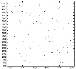
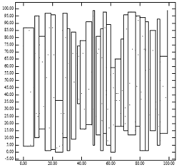
Figure 1 highlights the problem of the lowx packed R-tree. Figure 1 shows the leaf nodes of the R-tree that the lowx packing method will create for the points of Figure 1 . The fact that the resulting father nodes cover little area explains why the lowx packed R-tree achieves excellent performance for point queries. However, the fact that the fathers have large perimeters explains the degradation of performance for region queries. This is consistent with the analytical formulas for R-tree performance. Intuitively, the packing algorithm should ideally assign nearby points to the same leaf node. Ignorance of the y coordinate by the lowx packed R-tree tends to violate this empirical rule.
Figure 1: 200 points uniformly distributed; MBR of nodes generated by the "lowx packed R-tree" algorithm
The section below describes two variants of the Hilbert R-trees. The first index is suitable for the static database in which updates are very rare or in which there are no updates at all. The nodes of the resulting R-tree will be fully packed, with the possible exception of the last node at each level. Thus, the space utilization is ≈100%; this structure is called a packed Hilbert R-tree. The second index, called a Dynamic Hilbert R-tree, supports insertions and deletions, and is suitable for a dynamic environment.
Packed Hilbert R-trees
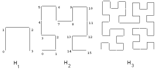
The following provides a brief introduction to the Hilbert curve. The basic Hilbert curve on a 2x2 grid, denoted by H1 is shown in Figure 2. To derive a curve of order i, each vertex of the basic curve is replaced by the curve of order i – 1, which may be appropriately rotated and/or reflected. Figure 2 also shows the Hilbert curves of order two and three. When the order of the curve tends to infinity, like other space filling curves, the resulting curve is a fractal, with a fractal dimension of two. The Hilbert curve can be generalized for higher dimensionalities. Algorithms for drawing the two-dimensional curve of a given order can be found in and. An algorithm for higher dimensionalities is given in.
The path of a space filling curve imposes a linear ordering on the grid points; this path may be calculated by starting at one end of the curve and following the path to the other end. The actual coordinate values of each point can be calculated. However, for the Hilbert curve this is much harder than for example the Z-order curve. Figure 2 shows one such ordering for a 4x4 grid (see curve H2). For example, the point (0,0) on the H2 curve has a Hilbert value of 0, while the point (1,1) has a Hilbert value of 2. The Hilbert value of a rectangle is defined as the Hilbert value of its center.
Figure 2: Hilbert curves of order 1, 2, and 3
The Hilbert curve imposes a linear ordering on the data rectangles and then traverses the sorted list, assigning each set of C rectangles to a node in the R-tree. The final result is that the set of data rectangles on the same node will be close to each other in the linear ordering, and most likely in the native space; thus, the resulting R-tree nodes will have smaller areas. Figure 2 illustrates the intuitive reasons why our Hilbert-based methods will result in good performance. The data is composed of points (the same points as given in Figure 1). By grouping the points according to their Hilbert values, the MBRs of the resulting R-tree nodes tend to be small square-like rectangles. This indicates that the nodes will likely have small area and small perimeters. Small area values result in good performance for point queries; small area and small perimeter values lead to good performance for larger queries.
Algorithm Hilbert-Pack
(packs rectangles into an R-tree)
Step 1. Calculate the Hilbert value for each data rectangle
Step 2. Sort data rectangles on ascending Hilbert values
Step 3. /* Create leaf nodes (level l=0) */
- While (there are more rectangles)
- generate a new R-tree node
- assign the next C rectangles to this node
Step 4. /* Create nodes at higher level (l + 1) */
- While (there are > 1 nodes at level l)
- sort nodes at level l ≥ 0 on ascending creation time
- repeat Step 3
The assumption here is that the data are static or the frequency of modification is low. This is a simple heuristic for constructing an R-tree with ~100% space utilization which at the same time will have a good response time.
Dynamic Hilbert R-trees
The performance of R-trees depends on the quality of the algorithm that clusters the data rectangles on a node. Hilbert R-trees use space-filling curves, and specifically the Hilbert curve, to impose a linear ordering on the data rectangles. The Hilbert value of a rectangle is defined as the Hilbert value of its center.
Tree structure
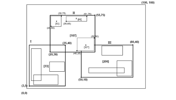
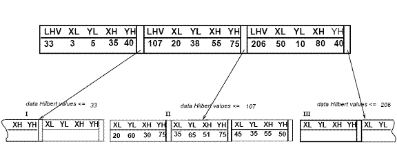
The Hilbert R-tree has the following structure. A leaf node contains at most Cl entries each of the form (R, obj _id) where Cl is the capacity of the leaf, R is the MBR of the real object (xlow, xhigh, ylow, yhigh) and obj-id is a pointer to the object description record. The main difference between the Hilbert R-tree and the R*-tree is that non-leaf nodes also contain information about the LHVs (Largest Hilbert Value). Thus, a non-leaf node in the Hilbert R-tree contains at most Cn entries of the form (R, ptr, LHV) where Cn is the capacity of a non-leaf node, R is the MBR that encloses all the children of that node, ptr is a pointer to the child node, and LHV is the largest Hilbert value among the data rectangles enclosed by R. Notice that since the non-leaf node picks one of the Hilbert values of the children to be the value of its own LHV, there is not extra cost for calculating the Hilbert values of the MBR of non-leaf nodes. Figure 3 illustrates some rectangles organized in a Hilbert R-tree. The Hilbert values of the centers are the numbers near the "x" symbols (shown only for the parent node "II"). The LHV's are in . Figure 4 shows how the tree of Figure 3 is stored on the disk; the contents of the parent node "II" are shown in more detail. Every data rectangle in node "I" has a Hilbert value v ≤33; similarly every rectangle in node "II" has a Hilbert value greater than 33 and ≤ 107, etc.
Figure 3: Data rectangles organized in a Hilbert R-tree (Hilbert values and largest Hilbert values (LHVs) are in Brackets)
A plain R-tree splits a node on overflow, creating two nodes from the original one. This policy is called a 1-to-2 splitting policy. It is possible also to defer the split, waiting until two nodes split into three. Note that this is similar to the B*-tree split policy. This method is referred to as the 2-to-3 splitting policy.
In general, this can be extended to s-to-(s+1) splitting policy; where s is the order of the splitting policy. To implement the order-s splitting policy, the overflowing node tries to push some of its entries to one of its s - 1 siblings; if all of them are full, then s-to-(s+1) split need to be done. The s -1 siblings are called the cooperating siblings.
Next, the algorithms for searching, insertion, and overflow handling are described in detail.
Searching
The searching algorithm is similar to the one used in other R-tree variants. Starting from the root, it descends the tree and examines all nodes that intersect the query rectangle. At the leaf level, it reports all entries that intersect the query window w as qualified data items.
Algorithm Search(node Root, rect w):
S1. Search nonleaf nodes:
- Invoke Search for every entry whose MBR intersects the query window w.
S2. Search leaf nodes:
- Report all entries that intersect the query window w as candidates.
Figure 4: The file structure for the Hilbert R-tree
Insertion
To insert a new rectangle r in the Hilbert R-tree, the Hilbert value h of the center of the new rectangle is used as a key. At each level the node with the minimum LHV value greater than h of all its siblings is chosen. When a leaf node is reached, the rectangle r is inserted in its correct order according to h. After a new rectangle is inserted in a leaf node N, AdjustTree is called to fix the MBR and largest Hilbert values in the upper-level nodes.
Algorithm Insert(node Root, rect r):
/* Inserts a new rectangle r in the Hilbert R-tree. h is the Hilbert value of the rectangle*/
I1. Find the appropriate leaf node:
- Invoke ChooseLeaf(r, h) to select a leaf node L in which to place r.
I2. Insert r in a leaf node L:
- If L has an empty slot, insert r in L in the
- appropriate place according to the Hilbert order and return.
- If L is full, invoke HandleOverflow(L,r), which
- will return new leaf if split was inevitable,
I3. Propagate changes upward:
- Form a set S that contains L, its cooperating siblings
- and the new leaf (if any)
- Invoke AdjustTree(S).
I4. Grow tree taller:
- If node split propagation caused the root to split, create
- a new root whose children are the two resulting nodes.
Algorithm ChooseLeaf(rect r, int h):
/* Returns the leaf node in which to place a new rectangle r. */
C1. Initialize:
- Set N to be the root node.
C2. Leaf check:
- If N is a leaf_ return N.
C3. Choose subtree:
- If N is a non-leaf node, choose the entry (R, ptr, LHV)
- with the minimum LHV value greater than h.
C4. Descend until a leaf is reached:
- Set N to the node pointed by ptr and repeat from C2.
Algorithm AdjustTree(set S):
/* S is a set of nodes that contains the node being updated, its cooperating siblings (if overflow has occurred) and the newly
created node NN (if split has occurred). The routine ascends from the leaf level towards the root, adjusting MBR and LHV of nodes that cover the nodes in S. It propagates splits (if any) */
A1. If root level is reached, stop.
A2. Propagate node split upward:
- Let Np be the parent node of N.
- If N has been split, let NN be the new node.
- Insert NN in Np in the correct order according to its Hilbert
- value if there is room. Otherwise, invoke HandleOverflow(Np , NN ).
- If Np is split, let PP be the new node.
A3. Adjust the MBR's and LHV's in the parent level:
- Let P be the set of parent nodes for the nodes in S.
- Adjust the corresponding MBR's and LHV's of the nodes in P appropriately.
A4. Move up to next level:
- Let S become the set of parent nodes P, with
- NN = PP, if Np was split.
- repeat from A1.
Deletion
In the Hilbert R-tree, there is no need to re-insert orphaned nodes whenever a father node underflows. Instead, keys can be borrowed from the siblings or the underflowing node is merged with its siblings. This is possible because the nodes have a clear ordering (according to Largest Hilbert Value, LHV); in contrast, in R-trees there is no such concept concerning sibling nodes. Notice that deletion operations require s cooperating siblings, while insertion operations require s - 1 siblings.
Algorithm Delete(r):
D1. Find the host leaf:
- Perform an exact match search to find the leaf node L
- that contains r.
D2. Delete r :
- Remove r from node L.
D3. If L underflows
- borrow some entries from s cooperating siblings.
- if all the siblings are ready to underflow.
- merge s + 1 to s nodes,
- adjust the resulting nodes.
D4. Adjust MBR and LHV in parent levels.
- form a set S that contains L and its cooperating
- siblings (if underflow has occurred).
- invoke AdjustTree(S).
Overflow handling
The overflow handling algorithm in the Hilbert R-tree treats the overflowing nodes either by moving some of the entries to one of the s - 1 cooperating siblings or by splitting s nodes into s +1 nodes.
Algorithm HandleOverflow(node N, rect r):
/* return the new node if a split occurred. */
H1. Let ε be a set that contains all the entries from N
- and its s - 1 cooperating siblings.
H2. Add r to ε.
H3. If at least one of the s - 1 cooperating siblings is not full,
- distribute ε evenly among the s nodes according to Hilbert values.
H4. If all the s cooperating siblings are full,
- create a new node NN and
- distribute ε evenly among the s + 1 nodes according
- to Hilbert values
- return NN.
Notes
- ^ I. Kamel and C. Faloutsos, On Packing R-trees, Second International ACM Conference on Information and Knowledge Management (CIKM), pages 490–499, Washington D.C., 1993.
- ^ H. Jagadish. Linear clustering of objects with multiple attributes. In Proc. of ACM SIGMOD Conf., pages 332–342, Atlantic City, NJ, May 1990.
- J. Griffiths. An algorithm for displaying a class of space-filling curves, Software-Practice and Experience 16(5), 403–411, May 1986.
- T. Bially. Space-filling curves. Their generation and their application to bandwidth reduction. IEEE Trans. on Information Theory. IT15(6), 658–664, November 1969.
- Beckmann, N.; Kriegel, H. P.; Schneider, R.; Seeger, B. (1990). "The R*-tree: an efficient and robust access method for points and rectangles". Proceedings of the 1990 ACM SIGMOD international conference on Management of data - SIGMOD '90 (PDF). p. 322. doi:10.1145/93597.98741. ISBN 0897913655. S2CID 11567855. Archived from the original (PDF) on 2018-04-17. Retrieved 2015-09-02.
References
- I. Kamel and C. Faloutsos. Parallel R-Trees. In Proc. of ACM SIGMOD Conf., pages 195–204 San Diego, CA, June 1992. Also available as Tech. Report UMIACS TR 92-1, CS-TR-2820.
- I. Kamel and C. Faloutsos. Hilbert R-tree: An improved R-tree using fractals. In Proc. of VLDB Conf., pages 500–509, Santiago, Chile, September 1994. Also available as Tech_ Report UMIACS TR 93-12.1 CS-TR-3032.1.
- N. Koudas, C. Faloutsos and I. Kamel. Declustering Spatial Databases on a Multi-Computer Architecture, International Conference on Extending Database Technology (EDBT), pages 592–614, 1996.
- N. Roussopoulos and D. Leifker. Direct spatial search on pictorial databases using Packed R-trees. In Proc. of ACM SIGMOD, pages 17–31, Austin, TX, May 1985.
- M. Schroeder. Fractals, Chaos, Power Laws: Minutes From an Infinite Paradise. W.H. Freeman and Company, NY, 1991.
- T. Sellis, N. Roussopoulos, and C. Faloutsos. The R+-Tree: a dynamic index for multi-dimensional objects. In Proc. 13th International Conference on VLDB, pages 507–518, England, September 1987.
| Tree data structures | |
|---|---|
| Search trees (dynamic sets/associative arrays) | |
| Heaps | |
| Tries | |
| Spatial data partitioning trees | |
| Other trees | |
| Data structures | |
|---|---|
| Types | |
| Abstract | |
| Arrays | |
| Linked | |
| Trees | |
| Graphs | |
