| This article includes a list of general references, but it lacks sufficient corresponding inline citations. Please help to improve this article by introducing more precise citations. (March 2011) (Learn how and when to remove this message) |

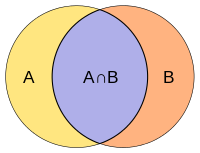
 Intersection and union of two sets A and B


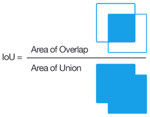
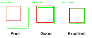
 Intersection over union as a similarity measure for object detection on images – an important task in computer vision.
The Jaccard index is a statistic used for gauging the similarity and diversity of sample sets. It is defined in general taking the ratio of two sizes (areas or volumes), the intersection size divided by the union size, also called intersection over union (IoU).
It was developed by Grove Karl Gilbert in 1884 as his ratio of verification (v) and now is often called the critical success index in meteorology. It was later developed independently by Paul Jaccard, originally giving the French name coefficient de communauté (community coefficient), and independently formulated again by T. Tanimoto. Thus, it is also called Tanimoto index or Tanimoto coefficient in some fields.
Overview
The Jaccard index measures similarity between finite sample sets and is defined as the size of the intersection divided by the size of the union of the sample sets:
Note that by design, If A intersection B is empty, then J(A, B) = 0. The Jaccard index is widely used in computer science, ecology, genomics, and other sciences, where binary or binarized data are used. Both the exact solution and approximation methods are available for hypothesis testing with the Jaccard index.
Jaccard similarity also applies to bags, i.e., multisets. This has a similar formula, but the symbols used represent bag intersection and bag sum (not union). The maximum value is 1/2.
The Jaccard distance, which measures dissimilarity between sample sets, is complementary to the Jaccard index and is obtained by subtracting the Jaccard index from 1 or, equivalently, by dividing the difference of the sizes of the union and the intersection of two sets by the size of the union:
An alternative interpretation of the Jaccard distance is as the ratio of the size of the symmetric difference to the union. Jaccard distance is commonly used to calculate an n × n matrix for clustering and multidimensional scaling of n sample sets.
This distance is a metric on the collection of all finite sets.
There is also a version of the Jaccard distance for measures, including probability measures. If is a measure on a measurable space , then we define the Jaccard index by
and the Jaccard distance by
Care must be taken if or , since these formulas are not well defined in these cases.
The MinHash min-wise independent permutations locality sensitive hashing scheme may be used to efficiently compute an accurate estimate of the Jaccard similarity index of pairs of sets, where each set is represented by a constant-sized signature derived from the minimum values of a hash function.
Similarity of asymmetric binary attributes
Given two objects, A and B, each with n binary attributes, the Jaccard index is a useful measure of the overlap that A and B share with their attributes. Each attribute of A and B can either be 0 or 1. The total number of each combination of attributes for both A and B are specified as follows:
- represents the total number of attributes where A and B both have a value of 1.
- represents the total number of attributes where the attribute of A is 0 and the attribute of B is 1.
- represents the total number of attributes where the attribute of A is 1 and the attribute of B is 0.
- represents the total number of attributes where A and B both have a value of 0.
| AB | 0 | 1 |
|---|---|---|
| 0 | ||
| 1 |
Each attribute must fall into one of these four categories, meaning that
The Jaccard similarity index, J, is given as
The Jaccard distance, dJ, is given as
Statistical inference can be made based on the Jaccard similarity index, and consequently related metrics. Given two sample sets A and B with n attributes, a statistical test can be conducted to see if an overlap is statistically significant. The exact solution is available, although computation can be costly as n increases. Estimation methods are available either by approximating a multinomial distribution or by bootstrapping.
Difference with the simple matching index (SMC)
When used for binary attributes, the Jaccard index is very similar to the simple matching coefficient. The main difference is that the SMC has the term in its numerator and denominator, whereas the Jaccard index does not. Thus, the SMC counts both mutual presences (when an attribute is present in both sets) and mutual absence (when an attribute is absent in both sets) as matches and compares it to the total number of attributes in the universe, whereas the Jaccard index only counts mutual presence as matches and compares it to the number of attributes that have been chosen by at least one of the two sets.
In market basket analysis, for example, the basket of two consumers who we wish to compare might only contain a small fraction of all the available products in the store, so the SMC will usually return very high values of similarities even when the baskets bear very little resemblance, thus making the Jaccard index a more appropriate measure of similarity in that context. For example, consider a supermarket with 1000 products and two customers. The basket of the first customer contains salt and pepper and the basket of the second contains salt and sugar. In this scenario, the similarity between the two baskets as measured by the Jaccard index would be 1/3, but the similarity becomes 0.998 using the SMC.
In other contexts, where 0 and 1 carry equivalent information (symmetry), the SMC is a better measure of similarity. For example, vectors of demographic variables stored in dummy variables, such as gender, would be better compared with the SMC than with the Jaccard index since the impact of gender on similarity should be equal, independently of whether male is defined as a 0 and female as a 1 or the other way around. However, when we have symmetric dummy variables, one could replicate the behaviour of the SMC by splitting the dummies into two binary attributes (in this case, male and female), thus transforming them into asymmetric attributes, allowing the use of the Jaccard index without introducing any bias. The SMC remains, however, more computationally efficient in the case of symmetric dummy variables since it does not require adding extra dimensions.
Weighted Jaccard similarity and distance
If and are two vectors with all real , then their Jaccard similarity index (also known then as Ruzicka similarity) is defined as
and Jaccard distance (also known then as Soergel distance)
With even more generality, if and are two non-negative measurable functions on a measurable space with measure , then we can define
where and are pointwise operators. Then Jaccard distance is
Then, for example, for two measurable sets , we have where and are the characteristic functions of the corresponding set.
Probability Jaccard similarity and distance
The weighted Jaccard similarity described above generalizes the Jaccard Index to positive vectors, where a set corresponds to a binary vector given by the indicator function, i.e. . However, it does not generalize the Jaccard Index to probability distributions, where a set corresponds to a uniform probability distribution, i.e.
It is always less if the sets differ in size. If , and then

Instead, a generalization that is continuous between probability distributions and their corresponding support sets is
which is called the "Probability" Jaccard. It has the following bounds against the Weighted Jaccard on probability vectors.
Here the upper bound is the (weighted) Sørensen–Dice coefficient. The corresponding distance, , is a metric over probability distributions, and a pseudo-metric over non-negative vectors.
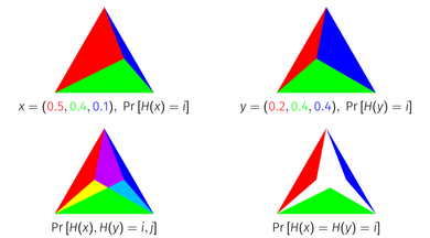
The Probability Jaccard Index has a geometric interpretation as the area of an intersection of simplices. Every point on a unit -simplex corresponds to a probability distribution on elements, because the unit -simplex is the set of points in dimensions that sum to 1. To derive the Probability Jaccard Index geometrically, represent a probability distribution as the unit simplex divided into sub simplices according to the mass of each item. If you overlay two distributions represented in this way on top of each other, and intersect the simplices corresponding to each item, the area that remains is equal to the Probability Jaccard Index of the distributions.
Optimality of the Probability Jaccard Index

Consider the problem of constructing random variables such that they collide with each other as much as possible. That is, if and , we would like to construct and to maximize . If we look at just two distributions in isolation, the highest we can achieve is given by where is the Total Variation distance. However, suppose we weren't just concerned with maximizing that particular pair, suppose we would like to maximize the collision probability of any arbitrary pair. One could construct an infinite number of random variables one for each distribution , and seek to maximize for all pairs . In a fairly strong sense described below, the Probability Jaccard Index is an optimal way to align these random variables.
For any sampling method and discrete distributions , if then for some where and , either or .
That is, no sampling method can achieve more collisions than on one pair without achieving fewer collisions than on another pair, where the reduced pair is more similar under than the increased pair. This theorem is true for the Jaccard Index of sets (if interpreted as uniform distributions) and the probability Jaccard, but not of the weighted Jaccard. (The theorem uses the word "sampling method" to describe a joint distribution over all distributions on a space, because it derives from the use of weighted minhashing algorithms that achieve this as their collision probability.)
This theorem has a visual proof on three element distributions using the simplex representation.
Tanimoto similarity and distance
Various forms of functions described as Tanimoto similarity and Tanimoto distance occur in the literature and on the Internet. Most of these are synonyms for Jaccard similarity and Jaccard distance, but some are mathematically different. Many sources cite an IBM Technical Report as the seminal reference.
In "A Computer Program for Classifying Plants", published in October 1960, a method of classification based on a similarity ratio, and a derived distance function, is given. It seems that this is the most authoritative source for the meaning of the terms "Tanimoto similarity" and "Tanimoto Distance". The similarity ratio is equivalent to Jaccard similarity, but the distance function is not the same as Jaccard distance.
Tanimoto's definitions of similarity and distance
In that paper, a "similarity ratio" is given over bitmaps, where each bit of a fixed-size array represents the presence or absence of a characteristic in the plant being modelled. The definition of the ratio is the number of common bits, divided by the number of bits set (i.e. nonzero) in either sample.
Presented in mathematical terms, if samples X and Y are bitmaps, is the ith bit of X, and are bitwise and, or operators respectively, then the similarity ratio is
If each sample is modelled instead as a set of attributes, this value is equal to the Jaccard index of the two sets. Jaccard is not cited in the paper, and it seems likely that the authors were not aware of it.
Tanimoto goes on to define a "distance" based on this ratio, defined for bitmaps with non-zero similarity:
This coefficient is, deliberately, not a distance metric. It is chosen to allow the possibility of two specimens, which are quite different from each other, to both be similar to a third. It is easy to construct an example which disproves the property of triangle inequality.
Other definitions of Tanimoto distance
Tanimoto distance is often referred to, erroneously, as a synonym for Jaccard distance . This function is a proper distance metric. "Tanimoto Distance" is often stated as being a proper distance metric, probably because of its confusion with Jaccard distance.
If Jaccard or Tanimoto similarity is expressed over a bit vector, then it can be written as
where the same calculation is expressed in terms of vector scalar product and magnitude. This representation relies on the fact that, for a bit vector (where the value of each dimension is either 0 or 1) then
and
This is a potentially confusing representation, because the function as expressed over vectors is more general, unless its domain is explicitly restricted. Properties of do not necessarily extend to . In particular, the difference function does not preserve triangle inequality, and is not therefore a proper distance metric, whereas is.
There is a real danger that the combination of "Tanimoto Distance" being defined using this formula, along with the statement "Tanimoto Distance is a proper distance metric" will lead to the false conclusion that the function is in fact a distance metric over vectors or multisets in general, whereas its use in similarity search or clustering algorithms may fail to produce correct results.
Lipkus uses a definition of Tanimoto similarity which is equivalent to , and refers to Tanimoto distance as the function . It is, however, made clear within the paper that the context is restricted by the use of a (positive) weighting vector such that, for any vector A being considered, Under these circumstances, the function is a proper distance metric, and so a set of vectors governed by such a weighting vector forms a metric space under this function.
Jaccard index in binary classification confusion matrices
In confusion matrices employed for binary classification, the Jaccard index can be framed in the following formula:
where TP are the true positives, FP the false positives and FN the false negatives.
See also
- Overlap coefficient
- Simple matching coefficient
- Hamming distance
- Sørensen–Dice coefficient, which is equivalent: and (: Jaccard index, : Sørensen–Dice coefficient)
- Tversky index
- Correlation
- Mutual information, a normalized metricated variant of which is an entropic Jaccard distance.
References
- Murphy, Allan H. (1996). "The Finley Affair: A Signal Event in the History of Forecast Verification". Weather and Forecasting. 11 (1): 3. Bibcode:1996WtFor..11....3M. doi:10.1175/1520-0434(1996)011<0003:TFAASE>2.0.CO;2. ISSN 1520-0434. S2CID 54532560.
- "Forecast Verification Glossary" (PDF). noaa.gov. Retrieved 21 May 2023.
- Jaccard, Paul (1901). "Étude comparative de la distribution florale dans une portion des Alpes et des Jura". Bulletin de la Société vaudoise des sciences naturelles (in French). 37 (142): 547–579.
- Jaccard, Paul (February 1912). "The Distribution of the Flora in the Alpine Zone.1". New Phytologist. 11 (2): 37–50. Bibcode:1912NewPh..11...37J. doi:10.1111/j.1469-8137.1912.tb05611.x. ISSN 0028-646X. S2CID 85574559.
- ^ Tanimoto TT (17 Nov 1958). "An Elementary Mathematical theory of Classification and Prediction". Internal IBM Technical Report. 1957 (8?).
- ^ Chung NC, Miasojedow B, Startek M, Gambin A (December 2019). "Jaccard/Tanimoto similarity test and estimation methods for biological presence-absence data". BMC Bioinformatics. 20 (Suppl 15): 644. arXiv:1903.11372. doi:10.1186/s12859-019-3118-5. PMC 6929325. PMID 31874610.
- Leskovec J, Rajaraman A, Ullman J (2020). Mining of Massive Datasets. Cambridge. ISBN 9781108476348. and p. 76–77 in an earlier version.
- Kosub S (April 2019). "A note on the triangle inequality for the Jaccard distance". Pattern Recognition Letters. 120: 36–38. arXiv:1612.02696. Bibcode:2019PaReL.120...36K. doi:10.1016/j.patrec.2018.12.007. S2CID 564831.
- ^ Lipkus AH (1999). "A proof of the triangle inequality for the Tanimoto distance". Journal of Mathematical Chemistry. 26 (1–3): 263–265. doi:10.1023/A:1019154432472. S2CID 118263043.
- Levandowsky M, Winter D (1971). "Distance between sets". Nature. 234 (5): 34–35. Bibcode:1971Natur.234...34L. doi:10.1038/234034a0. S2CID 4283015.
- ^ Moulton R, Jiang Y (2018). "Maximally Consistent Sampling and the Jaccard Index of Probability Distributions". 2018 IEEE International Conference on Data Mining (ICDM). pp. 347–356. arXiv:1809.04052. doi:10.1109/ICDM.2018.00050. ISBN 978-1-5386-9159-5. S2CID 49746072.
- For example Huihuan Q, Xinyu W, Yangsheng X (2011). Intelligent Surveillance Systems. Springer. p. 161. ISBN 978-94-007-1137-2.
- Rogers DJ, Tanimoto TT (October 1960). "A Computer Program for Classifying Plants". Science. 132 (3434): 1115–8. Bibcode:1960Sci...132.1115R. doi:10.1126/science.132.3434.1115. PMID 17790723.
- Aziz Taha, Abdel (2015). "Metrics for evaluating 3D medical image segmentation: analysis, selection, and tool". BMC Medical Imaging. 15 (29): 1–28. doi:10.1186/s12880-015-0068-x. PMC 4533825. PMID 26263899.
Further reading
- Tan PN, Steinbach M, Kumar V (2005). Introduction to Data Mining. Pearson Addison Wesley. ISBN 0-321-32136-7.
External links
- Introduction to Data Mining lecture notes from Tan, Steinbach, Kumar
- Kaggle Dstl Satellite Imagery Feature Detection - Evaluation
| Machine learning evaluation metrics | |
|---|---|
| Regression | |
| Classification | |
| Clustering | |
| Ranking | |
| Computer Vision | |
| NLP | |
| Deep Learning Related Metrics | |
| Recommender system | |
| Similarity | |

 If A intersection B is empty, then J(A, B) = 0. The Jaccard index is widely used in computer science, ecology, genomics, and other sciences, where

 to the union.
Jaccard distance is commonly used to calculate an n × n matrix for
  is a measure on a
  , then we define the Jaccard index by


 or
or  , since these formulas are not well defined in these cases.
 represents the total number of attributes where A and B both have a value of 1.
 represents the total number of attributes where the attribute of A is 0 and the attribute of B is 1.
 represents the total number of attributes where the attribute of A is 1 and the attribute of B is 0.
 represents the total number of attributes where A and B both have a value of 0.


 and
and  are two vectors with all real
  , then their Jaccard similarity index (also known then as Ruzicka similarity) is defined as


 and
and  are two non-negative measurable functions on a measurable space
 and
and  are pointwise operators. Then Jaccard distance is

 , we have
  where
where  and
and  are the characteristic functions of the corresponding set.
 . However, it does not generalize the Jaccard Index to probability distributions, where a set corresponds to a uniform probability distribution, i.e.

 , and
, and  then
then


 , is a metric over probability distributions, and a
  -simplex corresponds to a probability distribution on
  elements, because the unit
  and
and  , we would like to construct
  to maximize
  . If we look at just two distributions
  in isolation, the highest
  where
where  is the
  , and seek to maximize
  and discrete distributions
  then for some
  where
where  and
and  , either
  or
or  .
.
 on one pair without achieving fewer collisions than
  is the ith bit of X, and
  are
are  is
is


 . This function is a proper distance metric. "Tanimoto Distance" is often stated as being a proper distance metric, probably because of its confusion with Jaccard distance.


 does not preserve
  such that, for any vector A being considered,
  Under these circumstances, the function is a proper distance metric, and so a set of vectors governed by such a weighting vector forms a
 and
and  (
( : Jaccard index,
  : Sørensen–Dice coefficient)