Students of statistics and probability theory sometimes develop misconceptions about the normal distribution, ideas that may seem plausible but are mathematically untrue. For example, it is sometimes mistakenly thought that two linearly uncorrelated, normally distributed random variables must be statistically independent. However, this is untrue, as can be demonstrated by counterexample. Likewise, it is sometimes mistakenly thought that a linear combination of normally distributed random variables will itself be normally distributed, but again, counterexamples prove this wrong.
To say that the pair of random variables has a bivariate normal distribution means that every linear combination of and for constant (i.e. not random) coefficients and (not both equal to zero) has a univariate normal distribution. In that case, if and are uncorrelated then they are independent. However, it is possible for two random variables and to be so distributed jointly that each one alone is marginally normally distributed, and they are uncorrelated, but they are not independent; examples are given below.
Examples
A symmetric example

Suppose has a normal distribution with expected value 0 and variance 1. Let have the Rademacher distribution, so that or , each with probability 1/2, and assume is independent of . Let . Then and are uncorrelated, as can be verified by calculating their covariance. Moreover, both have the same normal distribution. And yet, and are not independent.
To see that and are not independent, observe that or that .
Finally, the distribution of the simple linear combination concentrates positive probability at 0: . Therefore, the random variable is not normally distributed, and so also and are not jointly normally distributed (by the definition above).
An asymmetric example

Suppose has a normal distribution with expected value 0 and variance 1. Let where is a positive number to be specified below. If is very small, then the correlation is near if is very large, then is near 1. Since the correlation is a continuous function of , the intermediate value theorem implies there is some particular value of that makes the correlation 0. That value is approximately 1.54. In that case, and are uncorrelated, but they are clearly not independent, since completely determines .
To see that is normally distributed—indeed, that its distribution is the same as that of —one may compute its cumulative distribution function:
where the next-to-last equality follows from the symmetry of the distribution of and the symmetry of the condition that .
In this example, the difference is nowhere near being normally distributed, since it has a substantial probability (about 0.88) of it being equal to 0. By contrast, the normal distribution, being a continuous distribution, has no discrete part—that is, it does not concentrate more than zero probability at any single point. Consequently and are not jointly normally distributed, even though they are separately normally distributed.
Examples with support almost everywhere in the plane
Suppose that the coordinates of a random point in the plane are chosen according to the probability density function Then the random variables and are uncorrelated, and each of them is normally distributed (with mean 0 and variance 1), but they are not independent.
It is well-known that the ratio of two independent standard normal random deviates and has a Cauchy distribution. One can equally well start with the Cauchy random variable and derive the conditional distribution of to satisfy the requirement that with and independent and standard normal. It follows that in which is a Rademacher random variable and is a Chi-squared random variable with two degrees of freedom.
Consider two sets of , . Note that is not indexed by – that is, the same Cauchy random variable is used in the definition of both and . This sharing of results in dependences across indices: neither nor is independent of . Nevertheless all of the and are uncorrelated as the bivariate distributions all have reflection symmetry across the axes.

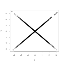
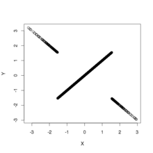
The figure shows scatterplots of samples drawn from the above distribution. This furnishes two examples of bivariate distributions that are uncorrelated and have normal marginal distributions but are not independent. The left panel shows the joint distribution of and ; the distribution has support everywhere but at the origin. The right panel shows the joint distribution of and ; the distribution has support everywhere except along the axes and has a discontinuity at the origin: the density diverges when the origin is approached along any straight path except along the axes.
See also
References
- ^ Rosenthal, Jeffrey S. (2005). "A Rant About Uncorrelated Normal Random Variables".
- ^ Melnick, Edward L.; Tenenbein, Aaron (November 1982). "Misspecifications of the Normal Distribution". The American Statistician. 36 (4): 372–373. doi:10.1080/00031305.1982.10483052.
- Hogg, Robert; Tanis, Elliot (2001). "Chapter 5.4 The Bivariate Normal Distribution". Probability and Statistical Inference (6th ed.). Prentice Hall. pp. 258–259. ISBN 0130272949.
- ^ Ash, Robert B. "Lecture 21. The Multivariate Normal Distribution" (PDF). Lectures on Statistics. Archived from the original (PDF) on 2007-07-14.
- Romano, Joesph P.; Siegel, Andrew F. (1986). Counterexamples in Probability and Statistics. Wadsworth & Brooks/Cole. pp. 65–66. ISBN 0-534-05568-0.
- Wise, Gary L.; Hall, Eric B. (1993). Counterexamples in Probability and Real Analysis. Oxford University Press. pp. 140–141. ISBN 0-19-507068-2.
- ^ Stoyanov, Jordan M. (2013). Counterexamples in Probability (3rd ed.). Dover. ISBN 978-0-486-49998-7.
- Patel, Jagdish K.; Read, Campbell B. (1996). Handbook of the Normal Distribution (2nd ed.). Taylor and Francis. p. 113. ISBN 978-0-824-79342-5.
- Krishnamoorthy, K. (2006). Handbook of Statistical Distributions with Applications. CRC Press. p. 278. ISBN 978-1-420-01137-1.
- Notes
- More precisely 1.53817..., the square root of the median of a chi-squared distribution with 3 degrees of freedom.
 of random variables has a
  of
of  and
and  for constant (i.e. not random) coefficients
  and
and  (not both equal to zero) has a univariate normal distribution. In that case, if
  have the
  or
or  , each with probability 1/2, and assume
  . Then
  or that
  .
.
 concentrates positive probability at 0:
  . Therefore, the random variable
  where
where  is a positive number to be specified below. If
  is near
  if
if 
 .
.
 is nowhere near being normally distributed, since it has a substantial probability (about 0.88) of it being equal to 0. By contrast, the normal distribution, being a continuous distribution, has no discrete part—that is, it does not concentrate more than zero probability at any single point. Consequently
  Then the random variables
  of two independent standard normal random deviates
  and
and  has a
has a  with
with  in which
  is a Rademacher random variable and
  is a
is a  ,
,  . Note that
  – that is, the same Cauchy random variable
  and
and  . This sharing of
  nor
nor  is independent of
  . Nevertheless all of the