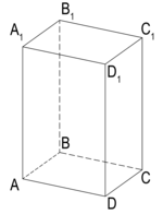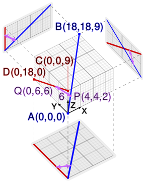
In three-dimensional geometry, skew lines are two lines that do not intersect and are not parallel. A simple example of a pair of skew lines is the pair of lines through opposite edges of a regular tetrahedron. Two lines that both lie in the same plane must either cross each other or be parallel, so skew lines can exist only in three or more dimensions. Two lines are skew if and only if they are not coplanar.
General position
If four points are chosen at random uniformly within a unit cube, they will almost surely define a pair of skew lines. After the first three points have been chosen, the fourth point will define a non-skew line if, and only if, it is coplanar with the first three points. However, the plane through the first three points forms a subset of measure zero of the cube, and the probability that the fourth point lies on this plane is zero. If it does not, the lines defined by the points will be skew.
Similarly, in three-dimensional space a very small perturbation of any two parallel or intersecting lines will almost certainly turn them into skew lines. Therefore, any four points in general position always form skew lines.
In this sense, skew lines are the "usual" case, and parallel or intersecting lines are special cases.
Formulas

Testing for skewness
Nearest points
See also: Line–line intersection § Nearest points to skew lines See also: Triangulation (computer vision) § Mid-point methodExpressing the two lines as vectors:
The cross product of and is perpendicular to the lines.
The plane formed by the translations of Line 2 along contains the point and is perpendicular to .
Therefore, the intersecting point of Line 1 with the above-mentioned plane, which is also the point on Line 1 that is nearest to Line 2 is given by
Similarly, the point on Line 2 nearest to Line 1 is given by (where )
Distance
The nearest points and form the shortest line segment joining Line 1 and Line 2:
The distance between nearest points in two skew lines may also be expressed using other vectors:
Here the 1×3 vector x represents an arbitrary point on the line through particular point a with b representing the direction of the line and with the value of the real number determining where the point is on the line, and similarly for arbitrary point y on the line through particular point c in direction d.
The cross product of b and d is perpendicular to the lines, as is the unit vector
The perpendicular distance between the lines is then
(if |b × d| is zero the lines are parallel and this method cannot be used).
More than two lines
See also: Line–line intersection § More than two linesConfigurations
A configuration of skew lines is a set of lines in which all pairs are skew. Two configurations are said to be isotopic if it is possible to continuously transform one configuration into the other, maintaining throughout the transformation the invariant that all pairs of lines remain skew. Any two configurations of two lines are easily seen to be isotopic, and configurations of the same number of lines in dimensions higher than three are always isotopic, but there exist multiple non-isotopic configurations of three or more lines in three dimensions. The number of nonisotopic configurations of n lines in R, starting at n = 1, is
Ruled surfaces

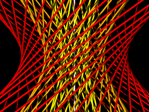
An affine transformation of this ruled surface produces a surface which in general has an elliptical cross-section rather than the circular cross-section produced by rotating L around L'; such surfaces are also called hyperboloids of one sheet, and again are ruled by two families of mutually skew lines. A third type of ruled surface is the hyperbolic paraboloid. Like the hyperboloid of one sheet, the hyperbolic paraboloid has two families of skew lines; in each of the two families the lines are parallel to a common plane although not to each other. Any three skew lines in R lie on exactly one ruled surface of one of these types.
Gallucci's theorem
If three skew lines all meet three other skew lines, any transversal of the first set of three meets any transversal of the second set.
Skew flats in higher dimensions
In higher-dimensional space, a flat of dimension k is referred to as a k-flat. Thus, a line may also be called a 1-flat.
Generalizing the concept of skew lines to d-dimensional space, an i-flat and a j-flat may be skew if i + j < d. As with lines in 3-space, skew flats are those that are neither parallel nor intersect.
In affine d-space, two flats of any dimension may be parallel. However, in projective space, parallelism does not exist; two flats must either intersect or be skew. Let I be the set of points on an i-flat, and let J be the set of points on a j-flat. In projective d-space, if i + j ≥ d then the intersection of I and J must contain a (i+j−d)-flat. (A 0-flat is a point.)
In either geometry, if I and J intersect at a k-flat, for k ≥ 0, then the points of I ∪ J determine a (i+j−k)-flat.
See also
References
- Weisstein, Eric W., "Line-Line Distance", MathWorld
- Viro, Julia Drobotukhina; Viro, Oleg (1990), "Configurations of skew lines" (PDF), Leningrad Math. J. (in Russian), 1 (4): 1027–1050, archived from the original (PDF) on 2021-11-09, retrieved 2006-10-24. Revised version in English: arXiv:math.GT/0611374
- Hilbert, David; Cohn-Vossen, Stephan (1952), Geometry and the Imagination (2nd ed.), Chelsea, pp. 13–17, ISBN 0-8284-1087-9
- Coxeter, H. S. M. (1969), Introduction to Geometry (2nd ed.), John Wiley & Sons, p. 257
- G. Gallucci (1906), "Studio della figura delle otto rette e sue applicazioni alla geometria del tetraedro ed alla teoria della configurazioni", Rendiconto dell'Accademia della Scienza Fisiche e Matematiche, 3rd series, 12: 49–79


 and
and  is perpendicular to the lines.

 contains the point
  and is perpendicular to
  .
.

 )
)

 and
and  form the shortest line segment joining Line 1 and Line 2:


 determining where the point is on the line, and similarly for arbitrary point y on the line through particular point c in direction d.

