In probability theory and statistics, complex random variables are a generalization of real-valued random variables to complex numbers, i.e. the possible values a complex random variable may take are complex numbers. Complex random variables can always be considered as pairs of real random variables: their real and imaginary parts. Therefore, the distribution of one complex random variable may be interpreted as the joint distribution of two real random variables.
Some concepts of real random variables have a straightforward generalization to complex random variables—e.g., the definition of the mean of a complex random variable. Other concepts are unique to complex random variables.
Applications of complex random variables are found in digital signal processing, quadrature amplitude modulation and information theory.
Definition
A complex random variable  on the probability space
  is a function
  such that both its real part
  and its imaginary part
  are real random variables on
  .
.
Examples
Simple example
Consider a random variable that may take only the three complex values  with probabilities as specified in the table. This is a simple example of a complex random variable.
Probability  |
Value 
|
 |

|
 |

|
 |

|
The expectation of this random variable may be simply calculated:

Uniform distribution
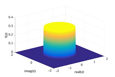
Another example of a complex random variable is the uniform distribution over the filled unit circle, i.e. the set  . This random variable is an example of a complex random variable for which the probability density function is defined. The density function is shown as the yellow disk and dark blue base in the following figure.

Complex normal distribution
Main article: Complex normal distribution
Complex Gaussian random variables are often encountered in applications. They are a straightforward generalization of real Gaussian random variables. The following plot shows an example of the distribution of such a variable.

Cumulative distribution function
The generalization of the cumulative distribution function from real to complex random variables is not obvious because expressions of the form  make no sense. However expressions of the form
  make sense. Therefore, we define the cumulative distribution
  of a complex random variables via the joint distribution of their real and imaginary parts:
 | | Eq.1 |
Probability density function
The probability density function of a complex random variable is defined as  , i.e. the value of the density function at a point
  is defined to be equal to the value of the joint density of the real and imaginary parts of the random variable evaluated at the point
  .
.
An equivalent definition is given by  where
where  and
and  .
.
As in the real case the density function may not exist.
Expectation
The expectation of a complex random variable is defined based on the definition of the expectation of a real random variable:
 | | Eq.2 |
Note that the expectation of a complex random variable does not exist if  or
or  does not exist.
If the complex random variable  has a probability density function
  , then the expectation is given by
  .
.
If the complex random variable  has a probability mass function
  , then the expectation is given by
  .
.
- Properties
Whenever the expectation of a complex random variable exists, taking the expectation and complex conjugation commute:

The expected value operator  is linear in the sense that

for any complex coefficients  even if
  and
and  are not independent.
Variance and pseudo-variance
The variance is defined in terms of absolute squares as:
![{\displaystyle \operatorname {K} _{ZZ}=\operatorname {Var} =\operatorname {E} \left\right|^{2}\right]=\operatorname {E} -\left|\operatorname {E} \right|^{2}}](https://wikimedia.org/api/rest_v1/media/math/render/svg/20d080a97d05f3891fad48566952956c8bc33616) | | Eq.3 |
- Properties
The variance is always a nonnegative real number. It is equal to the sum of the variances of the real and imaginary part of the complex random variable:

The variance of a linear combination of complex random variables may be calculated using the following formula:

Pseudo-variance
The pseudo-variance is a special case of the pseudo-covariance and is defined in terms of ordinary complex squares, given by:
![{\displaystyle \operatorname {J} _{ZZ}=\operatorname {E} )^{2}]=\operatorname {E} -(\operatorname {E} )^{2}}](https://wikimedia.org/api/rest_v1/media/math/render/svg/4ff6bdd87afbafd84fa355854e5d4d7884b7cb5f) | | Eq.4 |
Unlike the variance of  , which is always real and positive, the pseudo-variance of
  is in general complex.
Covariance matrix of real and imaginary parts
Further information: Complex random vector § Covariance matrices of real and imaginary parts
For a general complex random variable, the pair  has a covariance matrix of the form:

The matrix is symmetric, so 
Its elements equal:

Conversely:

Covariance and pseudo-covariance
The covariance between two complex random variables  is defined as
![{\displaystyle \operatorname {K} _{ZW}=\operatorname {Cov} =\operatorname {E} ){\overline {(W-\operatorname {E} )}}]=\operatorname {E} -\operatorname {E} \operatorname {E} }](https://wikimedia.org/api/rest_v1/media/math/render/svg/f7a961696e5eb2780adc679459b7cf2c5000dd1e) | | Eq.5 |
Notice the complex conjugation of the second factor in the definition.
In contrast to real random variables, we also define a pseudo-covariance (also called complementary variance):
![{\displaystyle \operatorname {J} _{ZW}=\operatorname {Cov} =\operatorname {E} )(W-\operatorname {E} )]=\operatorname {E} -\operatorname {E} \operatorname {E} }](https://wikimedia.org/api/rest_v1/media/math/render/svg/f0850e20d08a280f61bd0e8db2c108656c09f163) | | Eq.6 |
The second order statistics are fully characterized by the covariance and the pseudo-covariance.
- Properties
The covariance has the following properties:
 (Conjugate symmetry)
 (Sesquilinearity)


- Uncorrelatedness: two complex random variables
 and
and  are called uncorrelated if
  (see also: uncorrelatedness (probability theory)).
- Orthogonality: two complex random variables
 and
and  are called orthogonal if
  .
.
Circular symmetry
Circular symmetry of complex random variables is a common assumption used in the field of wireless communication. A typical example of a circular symmetric complex random variable is the complex Gaussian random variable with zero mean and zero pseudo-covariance matrix.
A complex random variable  is circularly symmetric if, for any deterministic
  , the distribution of
  equals the distribution of
  .
.
- Properties
By definition, a circularly symmetric complex random variable has
 for any
  .
.
Thus the expectation of a circularly symmetric complex random variable can only be either zero or undefined.
Additionally,
 for any
  .
.
Thus the pseudo-variance of a circularly symmetric complex random variable can only be zero.
If  and
and  have the same distribution, the phase of
  must be uniformly distributed over
  and independent of the amplitude of
  .
.
Proper complex random variables
The concept of proper random variables is unique to complex random variables, and has no correspondent concept with real random variables.
A complex random variable  is called proper if the following three conditions are all satisfied:


This definition is equivalent to the following conditions. This means that a complex random variable is proper if, and only if:


Theorem — Every circularly symmetric complex random variable with finite variance is proper.
For a proper complex random variable, the covariance matrix of the pair  has the following simple form:
 .
.
I.e.:

Cauchy-Schwarz inequality
The Cauchy-Schwarz inequality for complex random variables, which can be derived using the Triangle inequality and Hölder's inequality, is
 .
.
Characteristic function
The characteristic function of a complex random variable is a function  defined by

See also
References
- Eriksson, Jan; Ollila, Esa; Koivunen, Visa (2009). Statistics for complex random variables revisited. 2009 IEEE International Conference on Acoustics, Speech and Signal Processing. Taipei, Taiwan: Institute of Electrical and Electronics Engineers. pp. 3565–3568. doi:10.1109/ICASSP.2009.4960396.
- Lapidoth, A. (2009). A Foundation in Digital Communication. Cambridge University Press. ISBN 9780521193955.
- ^ Park,Kun Il (2018). Fundamentals of Probability and Stochastic Processes with Applications to Communications. Springer. ISBN 978-3-319-68074-3.
- Peter J. Schreier, Louis L. Scharf (2011). Statistical Signal Processing of Complex-Valued Data. Cambridge University Press. ISBN 9780511815911.
Categories:

 on the
  is a
is a  such that both its real part
  and its imaginary part
  are real
  with probabilities as specified in the table. This is a simple example of a complex random variable.


 . This random variable is an example of a complex random variable for which the

 make no sense. However expressions of the form
  make sense. Therefore, we define the cumulative distribution
  of a complex random variables via the
 , i.e. the value of the density function at a point
  is defined to be equal to the value of the joint density of the real and imaginary parts of the random variable evaluated at the point
  .
.
 where
where  and
and  .
.

 or
or  does not exist.
 , then the expectation is given by
  .
.
 , then the expectation is given by
  .
.

 is
is 
 even if
  are not
 ![{\displaystyle \operatorname {K} _{ZZ}=\operatorname {Var} =\operatorname {E} \left\right|^{2}\right]=\operatorname {E} -\left|\operatorname {E} \right|^{2}}](https://wikimedia.org/api/rest_v1/media/math/render/svg/20d080a97d05f3891fad48566952956c8bc33616)


![{\displaystyle \operatorname {J} _{ZZ}=\operatorname {E} )^{2}]=\operatorname {E} -(\operatorname {E} )^{2}}](https://wikimedia.org/api/rest_v1/media/math/render/svg/4ff6bdd87afbafd84fa355854e5d4d7884b7cb5f)
 has a
has a 


 is defined as
![{\displaystyle \operatorname {K} _{ZW}=\operatorname {Cov} =\operatorname {E} ){\overline {(W-\operatorname {E} )}}]=\operatorname {E} -\operatorname {E} \operatorname {E} }](https://wikimedia.org/api/rest_v1/media/math/render/svg/f7a961696e5eb2780adc679459b7cf2c5000dd1e)
![{\displaystyle \operatorname {J} _{ZW}=\operatorname {Cov} =\operatorname {E} )(W-\operatorname {E} )]=\operatorname {E} -\operatorname {E} \operatorname {E} }](https://wikimedia.org/api/rest_v1/media/math/render/svg/f0850e20d08a280f61bd0e8db2c108656c09f163)
 (Conjugate symmetry)
 (Sesquilinearity)


 (see also:
  .
. , the distribution of
  equals the distribution of
  for any
  .
.
 for any
  and independent of the amplitude of


 .
.
 .
. defined by
