Misplaced Pages

Normal-inverse-gamma distribution

Article snapshot taken from Wikipedia with creative commons attribution-sharealike license. Give it a read and then ask your questions in the chat. We can research this topic together.
(Redirected from Normal-inverse gamma distribution)
normal-inverse-gamma
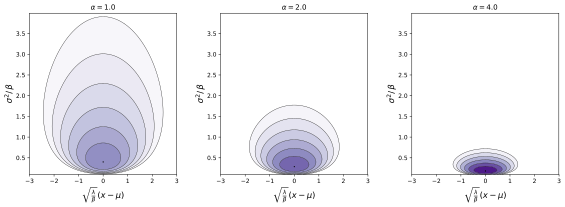
Probability density functionProbability density function of normal-inverse-gamma distribution for α = 1.0, 2.0 and 4.0, plotted in shifted and scaled coordinates.
Parameters μ {\displaystyle \mu \,} location (real)
λ > 0 {\displaystyle \lambda >0\,} (real)
α > 0 {\displaystyle \alpha >0\,} (real)
β > 0 {\displaystyle \beta >0\,} (real)
Support x ( , ) , σ 2 ( 0 , ) {\displaystyle x\in (-\infty ,\infty )\,\!,\;\sigma ^{2}\in (0,\infty )}
PDF λ 2 π σ 2 β α Γ ( α ) ( 1 σ 2 ) α + 1 exp ( 2 β + λ ( x μ ) 2 2 σ 2 ) {\displaystyle {\frac {\sqrt {\lambda }}{\sqrt {2\pi \sigma ^{2}}}}{\frac {\beta ^{\alpha }}{\Gamma (\alpha )}}\left({\frac {1}{\sigma ^{2}}}\right)^{\alpha +1}\exp \left(-{\frac {2\beta +\lambda (x-\mu )^{2}}{2\sigma ^{2}}}\right)}
Mean

E [ x ] = μ {\displaystyle \operatorname {E} =\mu }

E [ σ 2 ] = β α 1 {\displaystyle \operatorname {E} ={\frac {\beta }{\alpha -1}}} , for α > 1 {\displaystyle \alpha >1}
Mode

x = μ (univariate) , x = μ (multivariate) {\displaystyle x=\mu \;{\textrm {(univariate)}},x={\boldsymbol {\mu }}\;{\textrm {(multivariate)}}}

σ 2 = β α + 1 + 1 / 2 (univariate) , σ 2 = β α + 1 + k / 2 (multivariate) {\displaystyle \sigma ^{2}={\frac {\beta }{\alpha +1+1/2}}\;{\textrm {(univariate)}},\sigma ^{2}={\frac {\beta }{\alpha +1+k/2}}\;{\textrm {(multivariate)}}}
Variance

Var [ x ] = β ( α 1 ) λ {\displaystyle \operatorname {Var} ={\frac {\beta }{(\alpha -1)\lambda }}} , for α > 1 {\displaystyle \alpha >1}
Var [ σ 2 ] = β 2 ( α 1 ) 2 ( α 2 ) {\displaystyle \operatorname {Var} ={\frac {\beta ^{2}}{(\alpha -1)^{2}(\alpha -2)}}} , for α > 2 {\displaystyle \alpha >2}

Cov [ x , σ 2 ] = 0 {\displaystyle \operatorname {Cov} =0} , for α > 1 {\displaystyle \alpha >1}

In probability theory and statistics, the normal-inverse-gamma distribution (or Gaussian-inverse-gamma distribution) is a four-parameter family of multivariate continuous probability distributions. It is the conjugate prior of a normal distribution with unknown mean and variance.

Definition

Suppose

x σ 2 , μ , λ N ( μ , σ 2 / λ ) {\displaystyle x\mid \sigma ^{2},\mu ,\lambda \sim \mathrm {N} (\mu ,\sigma ^{2}/\lambda )\,\!}

has a normal distribution with mean μ {\displaystyle \mu } and variance σ 2 / λ {\displaystyle \sigma ^{2}/\lambda } , where

σ 2 α , β Γ 1 ( α , β ) {\displaystyle \sigma ^{2}\mid \alpha ,\beta \sim \Gamma ^{-1}(\alpha ,\beta )\!}

has an inverse-gamma distribution. Then ( x , σ 2 ) {\displaystyle (x,\sigma ^{2})} has a normal-inverse-gamma distribution, denoted as

( x , σ 2 ) N- Γ 1 ( μ , λ , α , β ) . {\displaystyle (x,\sigma ^{2})\sim {\text{N-}}\Gamma ^{-1}(\mu ,\lambda ,\alpha ,\beta )\!.}

( NIG {\displaystyle {\text{NIG}}} is also used instead of N- Γ 1 . {\displaystyle {\text{N-}}\Gamma ^{-1}.} )

The normal-inverse-Wishart distribution is a generalization of the normal-inverse-gamma distribution that is defined over multivariate random variables.

Characterization

Probability density function

f ( x , σ 2 μ , λ , α , β ) = λ σ 2 π β α Γ ( α ) ( 1 σ 2 ) α + 1 exp ( 2 β + λ ( x μ ) 2 2 σ 2 ) {\displaystyle f(x,\sigma ^{2}\mid \mu ,\lambda ,\alpha ,\beta )={\frac {\sqrt {\lambda }}{\sigma {\sqrt {2\pi }}}}\,{\frac {\beta ^{\alpha }}{\Gamma (\alpha )}}\,\left({\frac {1}{\sigma ^{2}}}\right)^{\alpha +1}\exp \left(-{\frac {2\beta +\lambda (x-\mu )^{2}}{2\sigma ^{2}}}\right)}

For the multivariate form where x {\displaystyle \mathbf {x} } is a k × 1 {\displaystyle k\times 1} random vector,

f ( x , σ 2 μ , V 1 , α , β ) = | V | 1 / 2 ( 2 π ) k / 2 β α Γ ( α ) ( 1 σ 2 ) α + 1 + k / 2 exp ( 2 β + ( x μ ) T V 1 ( x μ ) 2 σ 2 ) . {\displaystyle f(\mathbf {x} ,\sigma ^{2}\mid \mu ,\mathbf {V} ^{-1},\alpha ,\beta )=|\mathbf {V} |^{-1/2}{(2\pi )^{-k/2}}\,{\frac {\beta ^{\alpha }}{\Gamma (\alpha )}}\,\left({\frac {1}{\sigma ^{2}}}\right)^{\alpha +1+k/2}\exp \left(-{\frac {2\beta +(\mathbf {x} -{\boldsymbol {\mu }})^{T}\mathbf {V} ^{-1}(\mathbf {x} -{\boldsymbol {\mu }})}{2\sigma ^{2}}}\right).}

where | V | {\displaystyle |\mathbf {V} |} is the determinant of the k × k {\displaystyle k\times k} matrix V {\displaystyle \mathbf {V} } . Note how this last equation reduces to the first form if k = 1 {\displaystyle k=1} so that x , V , μ {\displaystyle \mathbf {x} ,\mathbf {V} ,{\boldsymbol {\mu }}} are scalars.

Alternative parameterization

It is also possible to let γ = 1 / λ {\displaystyle \gamma =1/\lambda } in which case the pdf becomes

f ( x , σ 2 μ , γ , α , β ) = 1 σ 2 π γ β α Γ ( α ) ( 1 σ 2 ) α + 1 exp ( 2 γ β + ( x μ ) 2 2 γ σ 2 ) {\displaystyle f(x,\sigma ^{2}\mid \mu ,\gamma ,\alpha ,\beta )={\frac {1}{\sigma {\sqrt {2\pi \gamma }}}}\,{\frac {\beta ^{\alpha }}{\Gamma (\alpha )}}\,\left({\frac {1}{\sigma ^{2}}}\right)^{\alpha +1}\exp \left(-{\frac {2\gamma \beta +(x-\mu )^{2}}{2\gamma \sigma ^{2}}}\right)}

In the multivariate form, the corresponding change would be to regard the covariance matrix V {\displaystyle \mathbf {V} } instead of its inverse V 1 {\displaystyle \mathbf {V} ^{-1}} as a parameter.

Cumulative distribution function

F ( x , σ 2 μ , λ , α , β ) = e β σ 2 ( β σ 2 ) α ( erf ( λ ( x μ ) 2 σ ) + 1 ) 2 σ 2 Γ ( α ) {\displaystyle F(x,\sigma ^{2}\mid \mu ,\lambda ,\alpha ,\beta )={\frac {e^{-{\frac {\beta }{\sigma ^{2}}}}\left({\frac {\beta }{\sigma ^{2}}}\right)^{\alpha }\left(\operatorname {erf} \left({\frac {{\sqrt {\lambda }}(x-\mu )}{{\sqrt {2}}\sigma }}\right)+1\right)}{2\sigma ^{2}\Gamma (\alpha )}}}

Properties

Marginal distributions

Given ( x , σ 2 ) N- Γ 1 ( μ , λ , α , β ) . {\displaystyle (x,\sigma ^{2})\sim {\text{N-}}\Gamma ^{-1}(\mu ,\lambda ,\alpha ,\beta )\!.} as above, σ 2 {\displaystyle \sigma ^{2}} by itself follows an inverse gamma distribution:

σ 2 Γ 1 ( α , β ) {\displaystyle \sigma ^{2}\sim \Gamma ^{-1}(\alpha ,\beta )\!}

while α λ β ( x μ ) {\displaystyle {\sqrt {\frac {\alpha \lambda }{\beta }}}(x-\mu )} follows a t distribution with 2 α {\displaystyle 2\alpha } degrees of freedom.

Proof for λ = 1 {\displaystyle \lambda =1}

For λ = 1 {\displaystyle \lambda =1} probability density function is

f ( x , σ 2 μ , α , β ) = 1 σ 2 π β α Γ ( α ) ( 1 σ 2 ) α + 1 exp ( 2 β + ( x μ ) 2 2 σ 2 ) {\displaystyle f(x,\sigma ^{2}\mid \mu ,\alpha ,\beta )={\frac {1}{\sigma {\sqrt {2\pi }}}}\,{\frac {\beta ^{\alpha }}{\Gamma (\alpha )}}\,\left({\frac {1}{\sigma ^{2}}}\right)^{\alpha +1}\exp \left(-{\frac {2\beta +(x-\mu )^{2}}{2\sigma ^{2}}}\right)}

Marginal distribution over x {\displaystyle x} is

f ( x μ , α , β ) = 0 d σ 2 f ( x , σ 2 μ , α , β ) = 1 2 π β α Γ ( α ) 0 d σ 2 ( 1 σ 2 ) α + 1 / 2 + 1 exp ( 2 β + ( x μ ) 2 2 σ 2 ) {\displaystyle {\begin{aligned}f(x\mid \mu ,\alpha ,\beta )&=\int _{0}^{\infty }d\sigma ^{2}f(x,\sigma ^{2}\mid \mu ,\alpha ,\beta )\\&={\frac {1}{\sqrt {2\pi }}}\,{\frac {\beta ^{\alpha }}{\Gamma (\alpha )}}\int _{0}^{\infty }d\sigma ^{2}\left({\frac {1}{\sigma ^{2}}}\right)^{\alpha +1/2+1}\exp \left(-{\frac {2\beta +(x-\mu )^{2}}{2\sigma ^{2}}}\right)\end{aligned}}}

Except for normalization factor, expression under the integral coincides with Inverse-gamma distribution

Γ 1 ( x ; a , b ) = b a Γ ( a ) e b / x x a + 1 , {\displaystyle \Gamma ^{-1}(x;a,b)={\frac {b^{a}}{\Gamma (a)}}{\frac {e^{-b/x}}{{x}^{a+1}}},}

with x = σ 2 {\displaystyle x=\sigma ^{2}} , a = α + 1 / 2 {\displaystyle a=\alpha +1/2} , b = 2 β + ( x μ ) 2 2 {\displaystyle b={\frac {2\beta +(x-\mu )^{2}}{2}}} .

Since 0 d x Γ 1 ( x ; a , b ) = 1 , 0 d x x ( a + 1 ) e b / x = Γ ( a ) b a {\displaystyle \int _{0}^{\infty }dx\Gamma ^{-1}(x;a,b)=1,\quad \int _{0}^{\infty }dxx^{-(a+1)}e^{-b/x}=\Gamma (a)b^{-a}} , and

0 d σ 2 ( 1 σ 2 ) α + 1 / 2 + 1 exp ( 2 β + ( x μ ) 2 2 σ 2 ) = Γ ( α + 1 / 2 ) ( 2 β + ( x μ ) 2 2 ) ( α + 1 / 2 ) {\displaystyle \int _{0}^{\infty }d\sigma ^{2}\left({\frac {1}{\sigma ^{2}}}\right)^{\alpha +1/2+1}\exp \left(-{\frac {2\beta +(x-\mu )^{2}}{2\sigma ^{2}}}\right)=\Gamma (\alpha +1/2)\left({\frac {2\beta +(x-\mu )^{2}}{2}}\right)^{-(\alpha +1/2)}}

Substituting this expression and factoring dependence on x {\displaystyle x} ,

f ( x μ , α , β ) x ( 1 + ( x μ ) 2 2 β ) ( α + 1 / 2 ) . {\displaystyle f(x\mid \mu ,\alpha ,\beta )\propto _{x}\left(1+{\frac {(x-\mu )^{2}}{2\beta }}\right)^{-(\alpha +1/2)}.}

Shape of generalized Student's t-distribution is

t ( x | ν , μ ^ , σ ^ 2 ) x ( 1 + 1 ν ( x μ ^ ) 2 σ ^ 2 ) ( ν + 1 ) / 2 {\displaystyle t(x|\nu ,{\hat {\mu }},{\hat {\sigma }}^{2})\propto _{x}\left(1+{\frac {1}{\nu }}{\frac {(x-{\hat {\mu }})^{2}}{{\hat {\sigma }}^{2}}}\right)^{-(\nu +1)/2}} .

Marginal distribution f ( x μ , α , β ) {\displaystyle f(x\mid \mu ,\alpha ,\beta )} follows t-distribution with 2 α {\displaystyle 2\alpha } degrees of freedom

f ( x μ , α , β ) = t ( x | ν = 2 α , μ ^ = μ , σ ^ 2 = β / α ) {\displaystyle f(x\mid \mu ,\alpha ,\beta )=t(x|\nu =2\alpha ,{\hat {\mu }}=\mu ,{\hat {\sigma }}^{2}=\beta /\alpha )} .

In the multivariate case, the marginal distribution of x {\displaystyle \mathbf {x} } is a multivariate t distribution:

x t 2 α ( μ , β α V ) {\displaystyle \mathbf {x} \sim t_{2\alpha }({\boldsymbol {\mu }},{\frac {\beta }{\alpha }}\mathbf {V} )\!}

Summation

Scaling

Suppose

( x , σ 2 ) N- Γ 1 ( μ , λ , α , β ) . {\displaystyle (x,\sigma ^{2})\sim {\text{N-}}\Gamma ^{-1}(\mu ,\lambda ,\alpha ,\beta )\!.}

Then for c > 0 {\displaystyle c>0} ,

( c x , c σ 2 ) N- Γ 1 ( c μ , λ / c , α , c β ) . {\displaystyle (cx,c\sigma ^{2})\sim {\text{N-}}\Gamma ^{-1}(c\mu ,\lambda /c,\alpha ,c\beta )\!.}

Proof: To prove this let ( x , σ 2 ) N- Γ 1 ( μ , λ , α , β ) {\displaystyle (x,\sigma ^{2})\sim {\text{N-}}\Gamma ^{-1}(\mu ,\lambda ,\alpha ,\beta )} and fix c > 0 {\displaystyle c>0} . Defining Y = ( Y 1 , Y 2 ) = ( c x , c σ 2 ) {\displaystyle Y=(Y_{1},Y_{2})=(cx,c\sigma ^{2})} , observe that the PDF of the random variable Y {\displaystyle Y} evaluated at ( y 1 , y 2 ) {\displaystyle (y_{1},y_{2})} is given by 1 / c 2 {\displaystyle 1/c^{2}} times the PDF of a N- Γ 1 ( μ , λ , α , β ) {\displaystyle {\text{N-}}\Gamma ^{-1}(\mu ,\lambda ,\alpha ,\beta )} random variable evaluated at ( y 1 / c , y 2 / c ) {\displaystyle (y_{1}/c,y_{2}/c)} . Hence the PDF of Y {\displaystyle Y} evaluated at ( y 1 , y 2 ) {\displaystyle (y_{1},y_{2})} is given by : f Y ( y 1 , y 2 ) = 1 c 2 λ 2 π y 2 / c β α Γ ( α ) ( 1 y 2 / c ) α + 1 exp ( 2 β + λ ( y 1 / c μ ) 2 2 y 2 / c ) = λ / c 2 π y 2 ( c β ) α Γ ( α ) ( 1 y 2 ) α + 1 exp ( 2 c β + ( λ / c ) ( y 1 c μ ) 2 2 y 2 ) . {\displaystyle f_{Y}(y_{1},y_{2})={\frac {1}{c^{2}}}{\frac {\sqrt {\lambda }}{\sqrt {2\pi y_{2}/c}}}\,{\frac {\beta ^{\alpha }}{\Gamma (\alpha )}}\,\left({\frac {1}{y_{2}/c}}\right)^{\alpha +1}\exp \left(-{\frac {2\beta +\lambda (y_{1}/c-\mu )^{2}}{2y_{2}/c}}\right)={\frac {\sqrt {\lambda /c}}{\sqrt {2\pi y_{2}}}}\,{\frac {(c\beta )^{\alpha }}{\Gamma (\alpha )}}\,\left({\frac {1}{y_{2}}}\right)^{\alpha +1}\exp \left(-{\frac {2c\beta +(\lambda /c)\,(y_{1}-c\mu )^{2}}{2y_{2}}}\right).\!}

The right hand expression is the PDF for a N- Γ 1 ( c μ , λ / c , α , c β ) {\displaystyle {\text{N-}}\Gamma ^{-1}(c\mu ,\lambda /c,\alpha ,c\beta )} random variable evaluated at ( y 1 , y 2 ) {\displaystyle (y_{1},y_{2})} , which completes the proof.

Exponential family

Normal-inverse-gamma distributions form an exponential family with natural parameters θ 1 = λ 2 {\displaystyle \textstyle \theta _{1}={\frac {-\lambda }{2}}} , θ 2 = λ μ {\displaystyle \textstyle \theta _{2}=\lambda \mu } , θ 3 = α {\displaystyle \textstyle \theta _{3}=\alpha } , and θ 4 = β + λ μ 2 2 {\displaystyle \textstyle \theta _{4}=-\beta +{\frac {-\lambda \mu ^{2}}{2}}} and sufficient statistics T 1 = x 2 σ 2 {\displaystyle \textstyle T_{1}={\frac {x^{2}}{\sigma ^{2}}}} , T 2 = x σ 2 {\displaystyle \textstyle T_{2}={\frac {x}{\sigma ^{2}}}} , T 3 = log ( 1 σ 2 ) {\displaystyle \textstyle T_{3}=\log {\big (}{\frac {1}{\sigma ^{2}}}{\big )}} , and T 4 = 1 σ 2 {\displaystyle \textstyle T_{4}={\frac {1}{\sigma ^{2}}}} .

Information entropy

Kullback–Leibler divergence

Measures difference between two distributions.

Maximum likelihood estimation

This section is empty. You can help by adding to it. (July 2010)

Posterior distribution of the parameters

See the articles on normal-gamma distribution and conjugate prior.

Interpretation of the parameters

See the articles on normal-gamma distribution and conjugate prior.

Generating normal-inverse-gamma random variates

Generation of random variates is straightforward:

  1. Sample σ 2 {\displaystyle \sigma ^{2}} from an inverse gamma distribution with parameters α {\displaystyle \alpha } and β {\displaystyle \beta }
  2. Sample x {\displaystyle x} from a normal distribution with mean μ {\displaystyle \mu } and variance σ 2 / λ {\displaystyle \sigma ^{2}/\lambda }

Related distributions

  • The normal-gamma distribution is the same distribution parameterized by precision rather than variance
  • A generalization of this distribution which allows for a multivariate mean and a completely unknown positive-definite covariance matrix σ 2 V {\displaystyle \sigma ^{2}\mathbf {V} } (whereas in the multivariate inverse-gamma distribution the covariance matrix is regarded as known up to the scale factor σ 2 {\displaystyle \sigma ^{2}} ) is the normal-inverse-Wishart distribution

See also

References

  1. Ramírez-Hassan, Andrés. 4.2 Conjugate prior to exponential family | Introduction to Bayesian Econometrics.
  • Denison, David G. T.; Holmes, Christopher C.; Mallick, Bani K.; Smith, Adrian F. M. (2002) Bayesian Methods for Nonlinear Classification and Regression, Wiley. ISBN 0471490369
  • Koch, Karl-Rudolf (2007) Introduction to Bayesian Statistics (2nd Edition), Springer. ISBN 354072723X
Probability distributions (list)
Discrete
univariate
with finite
support
with infinite
support
Continuous
univariate
supported on a
bounded interval
supported on a
semi-infinite
interval
supported
on the whole
real line
with support
whose type varies
Mixed
univariate
continuous-
discrete
Multivariate
(joint)
Directional
Univariate (circular) directional
Circular uniform
Univariate von Mises
Wrapped normal
Wrapped Cauchy
Wrapped exponential
Wrapped asymmetric Laplace
Wrapped Lévy
Bivariate (spherical)
Kent
Bivariate (toroidal)
Bivariate von Mises
Multivariate
von Mises–Fisher
Bingham
Degenerate
and singular
Degenerate
Dirac delta function
Singular
Cantor
Families
Categories: